
The Forcing Family: Turning Bidirectional Video DiTs into Streaming Generators
📅 Published: | 🔄 Updated:
📘 TABLE OF CONTENTS
- Part I — From Bidirectional Video DiTs to Streaming Generation
- Part II — Four Fundamental Mismatches
- 3. The Four Mismatches of Streaming Video Generation
- 3.1 Architectural Mismatch: Bidirectional Teacher vs. Causal Generator
- 3.2 State-Distribution Mismatch: Ground-Truth History vs. Generated History
- 3.3 Denoising-Trajectory Mismatch: Training Noise States vs. Streaming Inference
- 3.4 Horizon and Context Mismatch: Short Training vs. Long Deployment
- 3.5 A Unified View: Aligning the Deployment State
- 3. The Four Mismatches of Streaming Video Generation
- Part III — Four Technical Routes of the Forcing Family
- 4. Route I — Resolving Architectural Mismatch
- 4.1 The Problem with Direct Bidirectional-to-Causal Conversion
- 4.2 CausVid: Separating the Teacher's Judgment from the Student's Execution
- 4.3 Why a Bidirectional Teacher Is Not Automatically a Causal Teacher
- 4.4 Causal Forcing: Making the Initialization Target Observable
- 4.5 Causal Forcing++ and Causal-rCM: Few-Step Capability as an Initialization Requirement
- 4.6 What This Route Solves—and What Remains
- 5. Route II — Resolving State-Distribution Mismatch
- 5.1 Teacher Forcing and Exposure Bias
- 5.2 Self Forcing: Training on the Model's Own History
- 5.3 Self-Generated Errors as Training Signals
- 5.4 Resampling Forcing: Model-Dependent History without Identical Rollout Training
- 5.5 Clean, Self-Generated, and Resampled History as Different Design Choices
- 5.6 Connection to On-Policy Learning
- 5.7 Self-Aligned Forcing: History Is Also a Differentiable Representation
- 5.8 Elastic Forcing: State Alignment Does Not Require a Score Teacher
- 6. Route III — Resolving Denoising-Trajectory Mismatch
- 6.1 Why Strict Autoregressive Denoising Can Be Restrictive
- 6.2 Diffusion Forcing: A Two-Dimensional View of Time and Noise
- 6.3 Autoregression and Full Diffusion as Two Extremes
- 6.4 Rolling Forcing: Sharing a Region of Local Revision
- 6.5 Global Output Causality with Local Joint Denoising
- 6.6 Stream Forcing: Coverage and Deployment Alignment Must Be Balanced
- 6.7 Flex-Forcing: Causality as a Configurable Generation Regime
- 6.8 From Strict AR to Flexible Spatiotemporal Denoising
- 7. Route IV — Resolving Horizon and Context Mismatch
- 7.1 Why Infinite Execution Is Not Long-Horizon Competence
- 7.2 Error Accumulation and Temporal Drift
- 7.3 KV Cache Growth and Finite Memory
- 7.4 LongLive and Self-Forcing++: Train on the Horizon Where Failures Occur
- 7.5 Context Forcing and LongTake: Extend What the Supervisor Can Know
- 7.6 Reward Forcing: Consistency Must Leave Room for Motion
- 7.7 Slow Memory, Fast Memory, and Deliberate Retrieval
- 7.8 KV Compression, Sparse Attention, and Cache-Oriented Forcing
- 7.9 From Long Video Generation to Persistent World State
- 4. Route I — Resolving Architectural Mismatch
- Part IV — A Unified Perspective
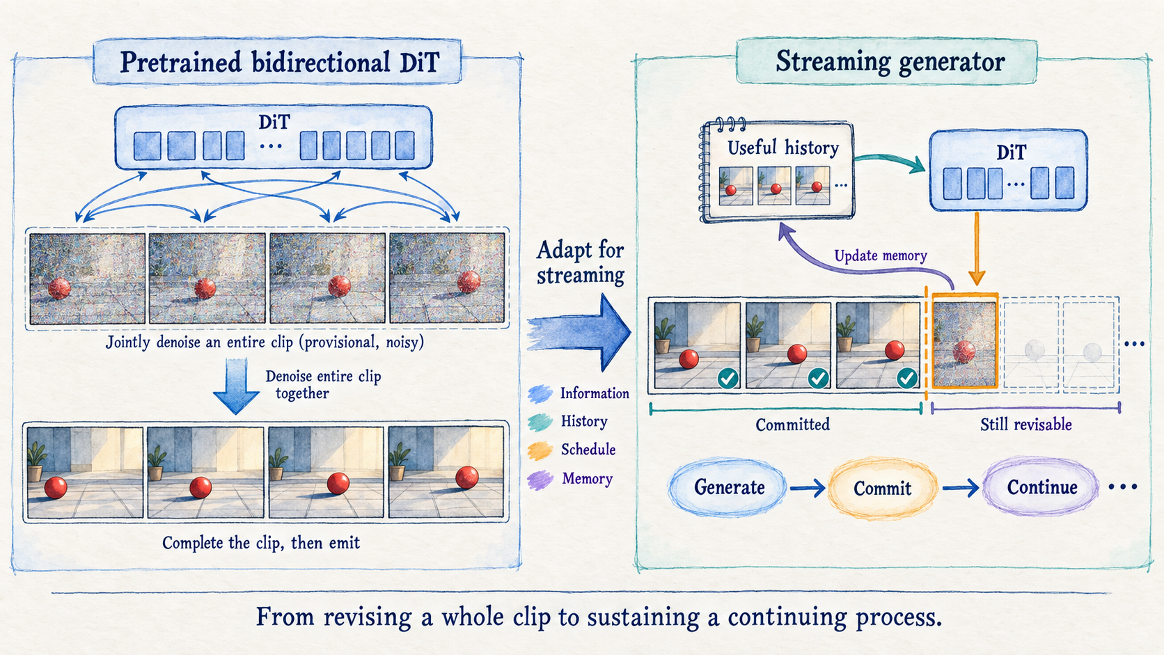
A pretrained video diffusion transformer can produce a compelling five-second clip because it is allowed to negotiate the entire clip before showing any of it. The opening pose can be revised to fit the ending; an object’s appearance can be reconciled across frames; motion can be coordinated using information from both temporal directions. Streaming removes this freedom. Once a frame has been displayed, the generator has to live with it.
That change explains much of the recent proliferation of forcing methods. The central difficulty is not merely replacing full attention with a causal mask or reducing the number of denoising steps. It is preserving the competence of a model trained to revise a complete video while asking it to make progressively irreversible decisions under a changing prompt, imperfect history, and finite memory.
My organizing claim is that the forcing family is best understood as an effort to align the learning problem with the actual state of a deployed streaming generator. Four mismatches make this alignment difficult: the teacher and student’s information structures, the provenance of historical states, the geometry of the denoising schedule, and the span and representation of memory. They give us four technical routes, but not four disjoint boxes. The most useful methods usually work across their boundaries.
The discussion below follows these routes rather than recounting algorithms. Named methods serve as evidence for changes in the underlying problem formulation. The scope is general streaming video diffusion, centered on converting pretrained bidirectional DiTs, with native causal training and interactive world modeling included where they clarify the limits of that conversion.
Part I — From Bidirectional Video DiTs to Streaming Generation
The conversion problem begins with a change in what the model is allowed to revise. A bidirectional DiT can coordinate an entire clip before committing any output, whereas a streaming generator must make useful decisions from a growing prefix. To understand what can be preserved under this constraint, we first examine the original generation regime, then construct a causal, teacher-forced baseline. That baseline will make the later mismatches concrete.
1. Bidirectional Video Generation and Its Streaming Limitation
Bidirectional generation owes much of its coherence to the ability to revise neighboring frames together. The same freedom that helps resolve motion and appearance also delays commitment, because the beginning of the clip remains coupled to unfinished future states. Understanding this coupling is the starting point for conversion: it tells us which benefits come from modeling the video distribution and which depend on a sampling process that a streaming system cannot retain unchanged.
1.1 Bidirectional Temporal Modeling in Video DiTs
Let $x^{1:N}$ denote a video in latent space, and let $c$ denote its conditioning. A bidirectional denoiser processes a noisy version of the entire sequence,
\[z^{1:N}_{\lambda}=\alpha(\lambda)x^{1:N}+\sigma(\lambda)\epsilon^{1:N},\]with a common noise level $\lambda$. Throughout this article, larger $\lambda$ means more noise, and $\lambda=0$ means clean. This convention also lets us discuss flow-based video models without depending on whether a particular implementation predicts noise, a clean sample, or velocity.
Temporal bidirectionality means that the prediction at position $i$ can use noisy states at positions both before and after $i$. The model is not observing the true future during generation: those future states are provisional samples that it helps construct. Nevertheless, they provide information that a generator operating on a committed prefix does not possess in the same form.
This is a powerful arrangement for joint synthesis. It allows the model to redistribute inconsistency across the clip instead of assigning every inconsistency to the next frame. Turning such a model into a streaming generator changes that allocation of responsibility.
1.2 Fixed-Length Full-Sequence Video Generation
A full-sequence model treats the whole active clip as revisable until sampling finishes. Its effective planning horizon and its output delay are therefore linked: to finalize the beginning, it generally has to process representations of the rest of the clip.
The fixed length is partly a training and systems choice, not a theorem about diffusion. Longer sequences can sometimes be sampled through extensions, overlapping windows, or alternative positional schemes. But those interventions do not automatically produce low-latency interaction. A system can generate a long video while still requiring substantial future computation before releasing its first frame.
For streaming, the important boundary is consequently commitment. Which outputs are final? Which internal states remain editable? How far ahead is the model computing? A duration benchmark cannot answer these questions on its own.
1.3 From Full-Sequence Generation to Causal Factorization
For a fixed conditioning sequence, the joint distribution admits the chain-rule factorization
\[p(x^{1:N}\mid c)=\prod_{i=1}^{N}p(x^i\mid x^{<i},c).\]There is no fundamental distributional contradiction between joint and autoregressive generation. In principle, both can represent the same distribution. The difficulty lies in learning an efficient causal sampler from a pretrained joint denoiser. Equality of endpoint distributions does not imply equality of sampling trajectories or equality of the information available at intermediate states.
For interactive generation, the conditioning itself arrives over time. The relevant transition becomes $p_\theta(x^i\mid x^{<i},c_{\leq i})$: future user actions are unavailable. This introduces an information constraint stronger than the chain rule for an offline video with a fully known prompt.
It is therefore misleading to write simply $p_{\mathrm{bi}}\neq p_{\mathrm{causal}}$ and infer that causal models must be inferior. A causal factorization can preserve a joint law; a restricted student may still fail to reproduce the particular teacher mapping used to supervise it.
1.4 Frame-wise and Chunk-wise Autoregressive Generation
Most practical systems operate on latent frames or chunks rather than individual decoded RGB frames. A temporally compressed video autoencoder can map one latent unit to several display frames. Statements about frame-wise response should be interpreted in that representation.
Chunk-wise autoregression keeps bidirectional computation inside a chunk while restricting dependencies between chunks. It offers a useful compromise: the model retains a small region for joint motion coordination, and the hardware processes more tokens in parallel. Smaller chunks reduce the amount of output committed before the next control update, but increase the number of autoregressive transitions per second of video.
The chunk size is thus more than a batching parameter. It determines the model’s local revision budget, the frequency with which its own errors become conditioning, and the temporal granularity at which an action can affect the stream.
1.5 What Streaming and Infinite-Length Generation Actually Require
A streaming generator must release usable output incrementally. A real-time generator must also keep up with playback under specified hardware and resolution. An interactive generator must respond quickly to new inputs. A long-horizon generator must maintain useful state after many transitions. These requirements overlap, but none implies all the others.
Three clocks help separate them: video time, which orders events in the scene; denoising time, which measures the uncertainty of latent states; and wall-clock time, which determines what the user experiences. A rolling schedule can improve the third by reorganizing the second across the first. That does not by itself guarantee faster response to a changed action.
Likewise, indefinite execution means the loop can continue under a bounded resource policy. It says nothing about whether the hundredth second still belongs to the same world. The goal is not an infinite list of frames. It is a stream whose past remains consequential without making its future rigid.
2. The Naive Baseline: Causal DiT with Teacher Forcing
Once generation is organized around a committed prefix, the most direct adaptation is to reuse the pretrained weights, restrict temporal attention, and train each new chunk against a clean data history. These choices make the conditional task well defined and expose a plausible path to streaming execution. They also separate the mechanics of becoming causal from the harder question of remaining reliable in deployment. We will use this baseline to trace where the training setup and the eventual generation loop begin to diverge.
2.1 Converting Bidirectional Attention into Causal Attention
The obvious starting point is to reuse the pretrained DiT weights, replace full temporal attention with a block-causal mask, and fine-tune the resulting model. Within the current chunk, tokens can interact freely; historical chunks provide context; future chunks are hidden.
This edit changes the computation even before any weights are updated. Features learned to combine evidence across the entire clip now have to make do with a prefix. A masked pretrained model is consequently an initialization for a new conditional task, not a completed conversion.
The causal mask also enables historical keys and values to be reused once their representations are fixed. But cache correctness requires more than temporal masking: the representation must remain compatible with the prompt, positional convention, and noise stage under which it is later read. These qualifications will matter as much as the mask itself.
2.2 Chunk-Based Autoregressive Video Generation
The baseline alternates between two operations: denoise a new chunk conditioned on historical chunks, then commit that chunk and make it available as history. Its generative model is
\[p_\theta(x^{1:K}\mid c)=\prod_{k=1}^{K}p_\theta(x^k\mid x^{<k},c),\]where $k$ now indexes chunks. Each conditional is itself a diffusion or flow-based generator.
This nested structure is valuable because it preserves the expressive continuous generation machinery of the pretrained model. It is also expensive: the next chunk usually waits for the current one to complete its denoising sequence. Causal attention removes a dependency on the rest of the video, but does not remove the sequential cost of multiple evaluations per chunk.
2.3 Teacher Forcing with Clean Historical Chunks
Teacher forcing supplies clean data prefixes while the current target is corrupted for denoising training. The model learns to predict a plausible continuation from a reliable reference. Proper masks and training layouts can expose many target chunks in one training computation without leaking their clean targets.
Here, teacher means the ground-truth history fed into the model. It does not necessarily mean a separate neural teacher used for distillation. Confusing these two meanings obscures much of the forcing literature.
This baseline provides a clear supervised conditional task. It also gives the model unusually favorable operating conditions: the preceding object is correctly shaped, its motion is coherent, and its appearance is consistent. During deployment, none of those properties is guaranteed by the prefix the model receives.
2.4 Training and Inference Pipelines
The essential distinction is compact enough to express without an algorithm:
\[\begin{aligned} \text{Training:}\quad &x^{<k}\sim p_{\mathrm{data}},\qquad z^k_\lambda\longrightarrow x^k,\\ \text{Inference:}\quad &\hat x^{<k}\sim p_\theta,\qquad \epsilon^k\longrightarrow \hat x^k. \end{aligned}\]Both pipelines have causal dependencies, yet they present different states to the same network. Deployment further introduces a sampler with a finite step budget, a cache policy, a decoding pipeline, and possibly changing controls. Those choices determine which states the model actually encounters.
This gives a useful rule for reading subsequent methods: distinguish the distribution of training inputs from the objective applied to those inputs. Training with a stronger distribution-matching loss does not automatically make the history representative of deployment. Generating one’s own history does not automatically make the supervising signal appropriate either.
2.5 Why the Naive Baseline Is Not Enough
Imagine a character walking behind a pillar and returning. The converted model needs to preserve the character without seeing the return in advance, continue from a slightly distorted self-generated walking pose, denoise under the actual streaming schedule, and retrieve the character’s appearance after it has left the recent window.
These are four different questions. Making the attention causal answers only part of the first. Increasing training robustness may answer part of the second. Overlapping denoising can improve the third. A larger cache addresses the fourth only if the model can use its contents.
The baseline therefore exposes four mismatches between the inherited learning setup and the intended deployment. Some originate in conversion; others already exist in short-clip pretraining and become more severe during streaming. The rest of the article maps each mismatch to the technical route that most directly addresses it.
Part II — Four Fundamental Mismatches
The causal baseline gives the generator a workable execution order, but execution order is only one part of the learning problem. Conversion also changes the information available to the model, the histories it encounters, the uncertain states it must denoise, and the context it can retain. Distinguishing these changes is essential: similar-looking drift can arise from different causes, and an intervention aimed at one cause may leave the others intact.
3. The Four Mismatches of Streaming Video Generation
The four mismatches can be located at four interfaces: between teacher and student, between training histories and generated histories, between supported denoising states and the deployed schedule, and between short visible context and persistent dependencies. Each interface asks a different alignment question. Examining them separately will let us identify what a method changes before judging whether it solves the failure seen in the stream.
3.1 Architectural Mismatch: Bidirectional Teacher vs. Causal Generator
Architectural mismatch is most precisely an information mismatch. A joint teacher can use the entire active noisy video. A strict autoregressive student sees a current noisy chunk and a prefix. An endpoint or update chosen by the teacher may depend on variables hidden from the student.
There are two consequences. First, simply masking the pretrained network changes the conditional denoising problem. Second, a paired distillation target may be impossible to reproduce as a deterministic function of the student’s inputs, even if the student can represent the teacher’s endpoint distribution through a different sampling construction.
The right diagnostic is therefore not only whether the two models have different attention masks. It is whether the supervision asks the student to use information that its deployment interface excludes.
3.2 State-Distribution Mismatch: Ground-Truth History vs. Generated History
Let $d_{\mathrm{data}}$ be the distribution of data prefixes used during training and $d^\pi_\theta$ the distribution of states visited by the generator under deployment procedure $\pi$. The latter depends on its sampler, rollout length, memory policy, and controls, not just its network weights.
Teacher forcing generally gives
\[d_{\mathrm{train}}(h)\neq d^\pi_\theta(h).\]A generated history is not merely a clean history plus independent Gaussian noise. It contains correlated modeling errors: an oversaturated region repeatedly reinforced, a pose that biases subsequent motion, or a background rearrangement that becomes accepted scene geometry. Exposure bias is the resulting failure to operate reliably on the states the model itself creates.
Notice that this problem remains even with a perfectly causal teacher. Matching who can see the future does not match who produced the past.
3.3 Denoising-Trajectory Mismatch: Training Noise States vs. Streaming Inference
A video diffusion state has both a temporal position and a noise level. We should therefore write a vector $\boldsymbol\lambda=(\lambda_1,\ldots,\lambda_W)$ for an active window, rather than assume that every frame has the same diffusion time.
Full-clip sampling usually advances the window at a shared noise level. Strict chunk autoregression combines completed history with one active noisy chunk. Rolling sampling can simultaneously maintain a nearly completed frame, a moderately noisy successor, and a largely unresolved future frame. Training on one of these configurations does not automatically prepare the model for the others.
The mismatch concerns more than a histogram of noise levels. It includes their cross-frame correlations, the sequence of transitions, the attention graph, and how noisy states become cache entries. A matched marginal distribution for each $\lambda_i$ can coexist with a badly mismatched joint trajectory.
3.4 Horizon and Context Mismatch: Short Training vs. Long Deployment
Long deployment introduces states absent from short training: large positional offsets, repeatedly reused history, cache eviction, prompt transitions, and dependencies whose evidence has disappeared from the active window. The numerical inequality $T_{\mathrm{train}}\ll T_{\mathrm{deploy}}$ describes only their surface manifestation.
There is also a supervision mismatch. A teacher assessing an isolated short segment can penalize local artifacts, but cannot reliably enforce facts that are visible only in distant history. Longer student rollouts expose the right failures; they do not automatically give the teacher the information needed to judge them.
This is why long-horizon stability needs both state coverage and supervision coverage. It may additionally need a memory representation capable of carrying the relevant facts. A model cannot retrieve what was evicted, and an objective cannot reward a dependency that it never observes.
3.5 A Unified View: Aligning the Deployment State
The deployed generator is better represented as a state transition system than as a bare denoiser. A useful conceptual state is
\[s_k=\left(m_k,\ z_{\mathcal A_k}^{\boldsymbol\lambda_k},\ c_{\leq k},\ \pi_k\right),\]where $m_k$ is historical memory, $\mathcal A_k$ is the active uncommitted region, and $\pi_k$ records the relevant scheduling and positional conventions. The four routes address, respectively, the permitted information in this transition, the provenance of its state, the evolution of its uncertainty, and the persistence of its memory.
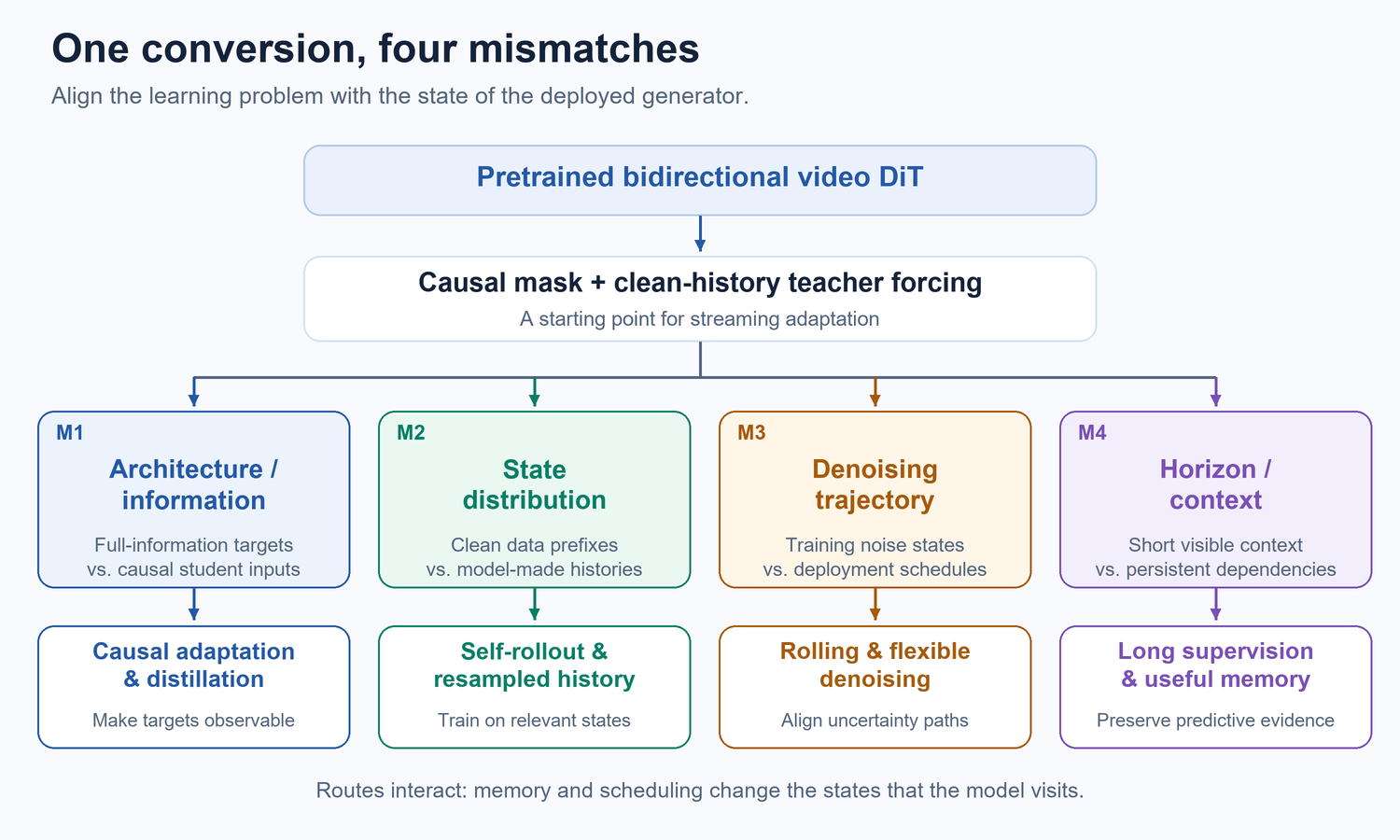
In this perspective, a compelling objective has the schematic form $\mathbb E_{s\sim d^\pi_\theta}[\ell(\theta;s)]$: evaluate the generator on states relevant to deployment. This is an organizing principle, not a proposed universal loss. Neither the state distribution nor the loss alone is sufficient; they must describe the same operating regime.
The next four chapters follow the branches in Figure 1. Each asks a different question: Is the target observable? Is the history representative? Is the denoising path supported? Is the remembered context sufficient?
Part III — Four Technical Routes of the Forcing Family
The four mismatches now give us a way to interpret the forcing family through the decisions each method changes. The first route makes supervision compatible with causal information; the second exposes the generator to its own states; the third reorganizes local denoising; and the fourth preserves useful context over time. We begin with supervision, because training on realistic histories cannot resolve a target that asks the student to reproduce choices based on information it never receives.
4. Route I — Resolving Architectural Mismatch
The first route concerns the target of conversion. It asks what a causal student should learn from a model whose native computation uses a complete clip. Its central principle is information-compatible supervision: matching a teacher’s distribution and copying its individual trajectories are different tasks.
4.1 The Problem with Direct Bidirectional-to-Causal Conversion
Suppose two complete noisy clips agree on the prefix visible to the student but contain different provisional futures. A joint denoiser may revise the current frame differently in the two clips. A strict causal student receives identical inputs in both cases. It cannot output two distinct deterministic revisions for the same input.
This is an observability problem before it is an optimization problem. More parameters or a more accurate regression fit cannot restore a hidden variable. The target must either be made conditional on the student’s information, be marginalized into a distribution that the student can sample, or be taught through an objective that does not require reproducing the inaccessible pairing.
The important limitation is specific. The student cannot reproduce an arbitrary full-information mapping after the inputs to that mapping have been projected away. It does not follow that the student cannot learn an equally rich causal video distribution.
4.2 CausVid: Separating the Teacher's Judgment from the Student's Execution
CausVid established an influential conversion pattern: a bidirectional diffusion teacher supervises a few-step causal student through asymmetric distribution matching, with teacher ODE trajectories used for initialization. The important abstraction is the separation between a strong model defining desirable video outputs and a streaming model implementing their generation.
A teacher can inspect a completed training rollout with information that will never be available to the student at inference. That is legitimate if it supplies a learning signal about the distribution of outputs. A critic of an entire performance need not perform it under the same conditions.
The qualification is that this asymmetry has different implications for different objectives. Distribution-level judgment can tolerate an asymmetric information structure. Direct regression to a particular teacher-generated endpoint may not. This distinction explains why asymmetric supervision can be useful while an initialization based on the same teacher can still be poorly aligned.
4.3 Why a Bidirectional Teacher Is Not Automatically a Causal Teacher
A simple statistical argument makes the issue tangible. Let $Y$ be the target selected using complete information, and let $I$ be the restricted information visible to the student. For deterministic squared-error regression,
\[\arg\min_g\mathbb E\left[\|g(I)-Y\|^2\right]=\mathbb E[Y\mid I].\]If $Y$ varies substantially after $I$ is fixed, the student learns an average over inaccessible choices. Consider a hand whose exact pose depends on an unseen future interaction. The average of several individually valid poses need not be a valid pose. This example is an illustration of conditional regression, not a claim that all diffusion training reduces to averaging images.
Noise in the student’s input does not remove the problem merely by being random. To reproduce a particular target, the target’s distinguishing information must be recoverable from the random variables the student actually receives. To match only a distribution, a different coupling between noise and output may be sufficient.
The design lesson is broader than video: a sample pairing can be harder to transfer than the distribution that produced the samples. Distillation should specify which of these objects it is trying to preserve.
4.4 Causal Forcing: Making the Initialization Target Observable
Causal Forcing diagnoses this issue in the ODE initialization of autoregressive students, using frame-level injectivity to analyze target ambiguity. Its intervention is to first obtain a causal diffusion teacher and use that teacher’s conditional trajectories for initialization. Subsequent refinement still uses asymmetric DMD. Thus it does not claim that every teacher in every training stage must be causal.
The useful high-level pattern is
\[\text{joint pretrained competence} \longrightarrow \text{causal conditional competence} \longrightarrow \text{fast causal execution}.\]Two compression problems have been separated: adapting the information structure and reducing the sampling budget. They interact, but solving both through a single poorly specified regression target makes their failures difficult to distinguish. This is also why a good initialization can matter after a powerful distribution-level refinement stage is added: refinement starts from the behaviors and state distribution that initialization has already created.
4.5 Causal Forcing++ and Causal-rCM: Few-Step Capability as an Initialization Requirement
The architectural question becomes more demanding when a chunk-wise four-step generator is pushed toward frame-wise one- or two-step operation. More transitions expose the model to its own mistakes more frequently, while fewer denoising evaluations leave less opportunity to refine each transition.
Causal Forcing++ uses causal consistency distillation to obtain an autoregressive few-step initialization without storing full teacher trajectories. Its conceptual contribution is to require the initial student to be causal, fast, and scalable at the same time. The paper studies one-, two-, and four-step settings; this should not be reduced to a universal claim of lossless one-step generation.
Causal-rCM further treats teacher-forcing consistency training and self-forcing DMD as complementary stages, including continuous-time consistency approaches for causal video models. This reinforces a more useful view than a contest between labels: reliable conditional training can establish a good starting transition, and rollout-based refinement can subsequently make that transition reliable on its own states.
My interpretation is that few-step capability belongs to the definition of the transition being initialized. A many-step causal model can be an excellent conditional denoiser while being a poor one-step state transition. Causality alone does not bridge that numerical gap.
4.6 What This Route Solves—and What Remains
This route makes the learned target compatible with the student’s information and intended step budget. It does not, by itself, ensure that the histories encountered during deployment were represented during training.
A causal teacher trained on pristine prefixes can still teach a student to depend on pristine prefixes. An excellent few-step conditional sampler can still repeatedly sharpen an artifact when its own output is fed back as context. Conversely, self-generated history cannot make an inaccessible paired target observable.
The two routes are therefore complementary interventions. The first improves what the transition is being asked to do. The second improves the states on which it is asked to do it. A robust system needs both, regardless of which method name appears on its checkpoint.
5. Route II — Resolving State-Distribution Mismatch
The second route concerns where history comes from. Its central problem is feedback: a prediction becomes the next input, so an error changes both the current video and the conditions under which the next prediction is made.
5.1 Teacher Forcing and Exposure Bias
Teacher forcing teaches continuations of data states. Deployment asks for continuations of model states. The gap can be small for the first chunk and substantial after dozens of transitions.
For example, a slight change in lighting may be acceptable in isolation. But if the next prediction treats that change as the new baseline and exaggerates it again, the stream gradually becomes overexposed. Training only on normally exposed prefixes gives little evidence about the behavior needed in that feedback loop.
This does not make teacher forcing a defective objective. With exact conditional learning, sufficient capacity, and complete data coverage, it can recover the desired joint distribution. Exposure bias matters because finite models have errors, and those errors move deployment into regions where their conditionals have not been learned reliably. The practical problem is reliable behavior under approximation.
5.2 Self Forcing: Training on the Model's Own History
Self Forcing places autoregressive self-rollout with KV caching inside training and supervises the generated video with a distribution-level objective. Few-step generation and stochastic gradient truncation make this practical. The defining change is the origin of the conditioning states: the student experiences its own earlier outputs when producing later ones.
This is more substantial than attaching a different loss to teacher-forced inputs. The model is evaluated inside the feedback loop it will inhabit at inference. It must produce outputs that remain useful as subsequent context, not merely outputs that look good when preceded by flawless data.
The distinction between sampling a state and differentiating through the path that created it remains important. Self-rollout can expose the relevant states even when gradients through parts of the rollout are truncated. That is not equivalent to optimizing the entire infinite-horizon process with full backpropagation.
5.3 Self-Generated Errors as Training Signals
The most useful interpretation is that generated errors identify the model’s fragile directions. Additive noise perturbs many directions that deployment may rarely visit. A generated malformed edge or drifting color exposes a direction the current model actually tends to reinforce.
However, learning from imperfect history does not necessarily mean reconstructing the ground-truth continuation of that history. Suppose a generated person turns left while the data person turns right. Both branches may be plausible. Supervising the generated left-turn state with the unchanged right-turn target would create an inconsistent task. Distributional or otherwise compatible supervision matters because self-generation can alter content, not just introduce small residual errors.
The desired property is continuation stability: remain visually and semantically plausible given the committed past, avoid amplifying incidental defects, and preserve the freedoms needed for the scene to evolve. The model cannot repair a frame already shown to the user. It can stop turning its defect into a permanent rule for future frames.
5.4 Resampling Forcing: Model-Dependent History without Identical Rollout Training
Resampling Forcing uses self-resampling of corrupted data videos to create histories containing model-dependent errors, followed by diffusion supervision with a sparse causal training layout. It is a teacher-free end-to-end training framework, with teacher-forcing warmup and history routing also part of its design. It is therefore broader than a cheaper implementation of Self Forcing.
The abstraction is to learn on a controlled neighborhood of data states shaped by the model’s own reconstruction behavior. This retains a connection to paired real-video supervision while exposing imperfections that simple Gaussian corruption may miss.
Such histories should be called model-dependent surrogates, not exactly on-policy histories. They remain anchored to a source video and a chosen resampling strength. Their advantages and limits depend on whether that neighborhood covers the errors the deployed free-running model actually makes. Cost savings alone do not establish distributional equivalence.
5.5 Clean, Self-Generated, and Resampled History as Different Design Choices
The three regimes can be summarized without treating them as a mandatory chronology:
| History source | What it provides | Main limitation |
|---|---|---|
| Clean data prefix | Accurate scene evidence and straightforward supervised targets | Limited coverage of the model’s own failure states |
| Free-running model prefix | States produced by the current rollout procedure | Sequential training work, drifting state distributions, and difficult long-range credit assignment |
| Model-resampled data prefix | Controlled, model-shaped imperfections near a reference trajectory | Approximation bias and dependence on resampling strength |
The choice is a trade-off among state realism, supervisory compatibility, and computational cost. Mixing regimes can be sensible. Early clean supervision establishes a usable transition; later model-dependent states reveal fragility. A model that cannot yet produce meaningful history offers little useful self-rollout signal.
There is also no general implication that the most realistic state distribution yields the easiest optimization. Hard states can be informative only if the loss can distinguish a correct continuation from an arbitrary departure.
5.6 Connection to On-Policy Learning
The analogy to on-policy learning is useful at the level of state visitation. Self-rollout obtains states from the current generator; teacher forcing obtains them from a different process. But teacher forcing is not literally an off-policy reinforcement-learning estimator, and Self Forcing is not automatically policy-gradient reinforcement learning.
The relevant conceptual objective is
\[\mathcal J(\theta;\pi)=\mathbb E_{h\sim d^\pi_\theta}\left[\ell_\theta(h)\right].\]The parameter $\theta$ affects both the transition loss and the state distribution. Truncating gradients through historical generation changes the credit-assignment approximation; it does not erase the value of sampling representative states. This distinction is essential when comparing training methods that all claim to match inference.
It also explains why deployment changes can reopen the gap. A new chunk size, aggressive quantization, a different cache policy, or a lower denoising budget can change $d^\pi_\theta$ even when the weights stay fixed. On-policy alignment is always relative to an operating procedure.
5.7 Self-Aligned Forcing: History Is Also a Differentiable Representation
The late-September Self-Aligned Forcing shows why the history problem cannot be described only by the pixels that were generated. It aligns historical K/V representations with the current denoising stage and allows future losses to differentiate through history encoding within the supervised stage. It retains self-rollout with stage-wise gradient truncation and a clean persistent sink; it does not restore unrestricted backpropagation through every denoising step.
The broader implication is that a historical chunk serves two roles: it is displayed content, and it is a representation written for future consumption. Those roles need not have the same optimum. A feature that improves the current chunk may be a poor summary for predicting subsequent motion.
This motivates a distinction between learning to read imperfect memory and learning to write useful memory. Detached caches emphasize the former. Differentiable history encoding can provide the latter as well. It is a credit-assignment dimension that crosses the state, trajectory, and context routes.
5.8 Elastic Forcing: State Alignment Does Not Require a Score Teacher
Elastic Forcing, first released on September 28, replaces auxiliary diffusion score models during post-training with reference-video distribution matching in frozen video representation spaces using MMD. Its reported setup reuses a pretrained architecture and initialization; teacher-free post-training should not be confused with training the entire system without pretrained knowledge. Its main feature-distribution objective also does not inherently guarantee exact prompt-conditional matching.
The simultaneous September 30 work Radian takes a complementary direction: representation-space adversarial supervision from real videos supplements on-policy DMD rather than replacing it.
Taken together, these works separate two questions that were previously often bundled: Which states should the student visit, and what evidence should judge its outputs? A self-generated rollout can be judged by a diffusion teacher, reference samples, a learned critic, rewards, or combinations of these. Each changes the target and the blind spots of supervision; none removes the need for representative histories.
6. Route III — Resolving Denoising-Trajectory Mismatch
Route II asks who produced the history. Route III asks how uncertainty is distributed and resolved across the active video. Generated history can be paired with a strict autoregressive schedule, a rolling schedule, or a flexible one. They are separate choices, even when a method changes both.
6.1 Why Strict Autoregressive Denoising Can Be Restrictive
Strict chunk autoregression completely resolves the current chunk before beginning its successor. This creates a simple execution graph and permits clean historical caching. But it allocates the entire refinement budget to one local commitment at a time.
Consider two neighboring chunks describing a hand moving onto a table. A jointly revisable region can coordinate the approach and the contact before either is finalized. A strict sequential generator must place the approach first and make the contact compatible afterward. If the approach is slightly wrong, the successor has fewer ways to reconcile it.
This is a limitation of the available revision region, not proof that autoregression necessarily accumulates errors. An accurate causal transition can remain stable. The argument for rolling denoising is that local mutual refinement may be an easier use of inherited bidirectional competence than demanding perfect sequential commitments at very fine granularity.
6.2 Diffusion Forcing: A Two-Dimensional View of Time and Noise
Diffusion Forcing introduced independent per-token noise levels as a sequence-training paradigm, combining next-token prediction with full-sequence denoising capabilities. Its foundational formulation was broader than the later conversion of pretrained video DiTs. The relevant inheritance is the idea that different temporal positions need not share a single diffusion time.
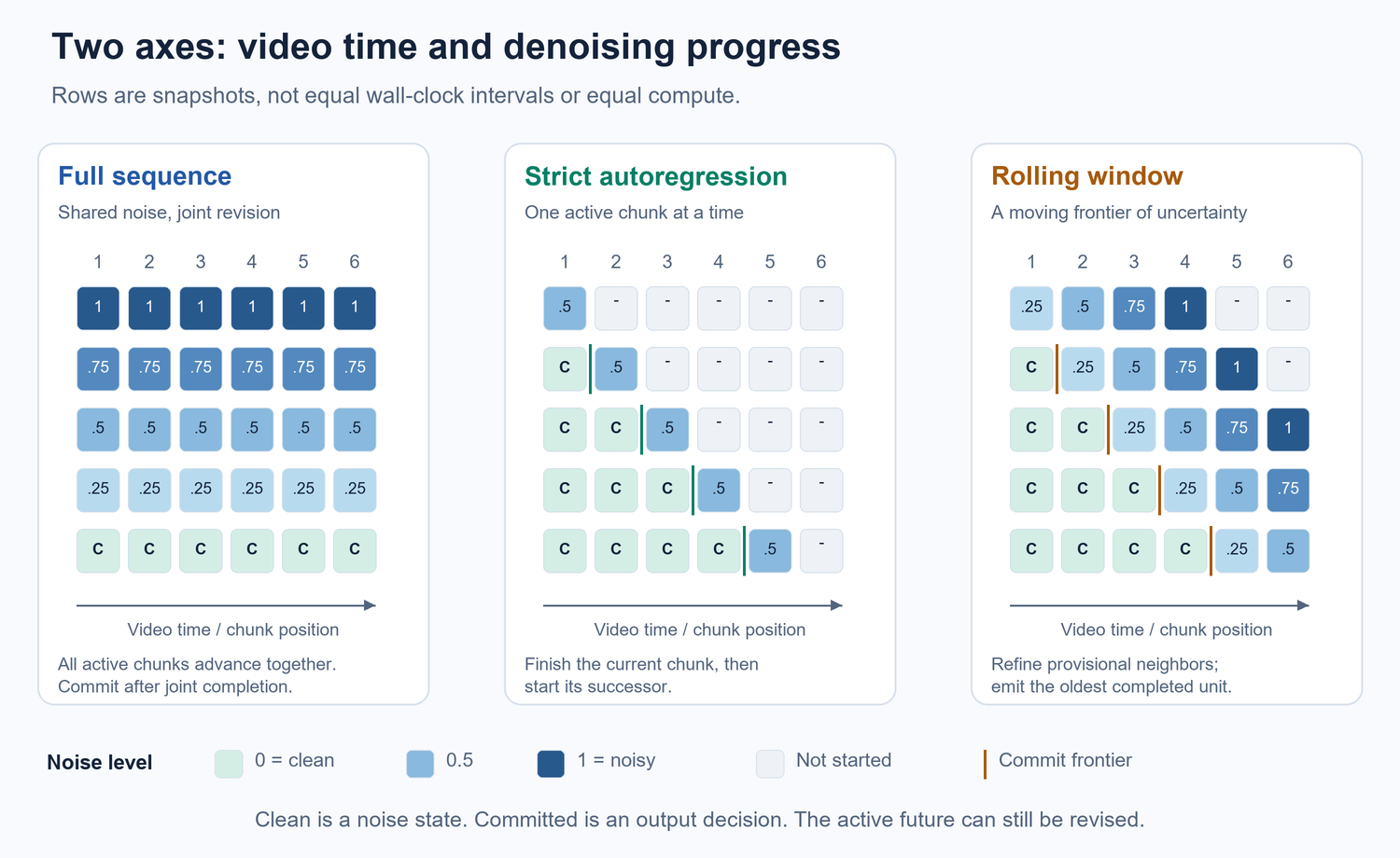
We can now visualize generation on a grid: temporal position is one axis, noise level the other. A sampler traces a path through this grid. It can finish one token before advancing, reduce uncertainty for many tokens together, or interleave progress across them.
This changes the meaning of historical information. History need not always be a completed sample; it may be a noisy representation carrying partial evidence. Training for such states can make the model more flexible, but only if inference uses compatible representations and transitions.
6.3 Autoregression and Full Diffusion as Two Extremes
The schedules have simple limiting forms. Full-sequence diffusion traverses the diagonal $\lambda_1=\cdots=\lambda_W$. Strict autoregression presents clean history, $\lambda_{<i}=0$, alongside one noisy current unit. A rolling window occupies a graded profile such as
\[0\leq\lambda_i<\lambda_{i+1}<\cdots<\lambda_{i+W-1}.\]These expressions specify noise configurations, not complete models. The attention graph must also be specified. A heterogeneous-noise model can have strictly causal attention; a rolling window can instead permit bidirectional attention among its unfinished states. Their representational capabilities differ even if their noise profiles look similar.
This distinction prevents an overly broad claim about Diffusion Forcing: learning to denoise many configurations supplies a vocabulary of uncertain states, but does not prescribe one universal streaming scheduler. Training coverage, access to future provisional latents, and emission order remain separate design dimensions.
History-Guided Video Diffusion, including the Diffusion Forcing Transformer and History Guidance, is a relevant bridge to transformer video models: it supports flexible history conditioning and controls how strongly history constrains generation. It illustrates that a noise level can govern the confidence assigned to context, as well as the amount of work remaining before a frame is finished. Flexible history conditioning alone does not imply an efficient causal KV-cached implementation.
6.4 Rolling Forcing: Sharing a Region of Local Revision
Rolling Forcing combines a rolling diffusion window with joint denoising of adjacent states at progressively increasing noise levels, self-generated historical conditioning, and persistent attention anchors. Within its active window, bidirectional interaction allows provisional neighboring frames to refine one another before emission.
The transferable insight is to distinguish the committed prefix from the uncommitted region. The prefix is a boundary condition. Inside the active region, the model can retain some of the cooperative computation that made the pretrained bidirectional network effective.
A rolling schedule also pipelines denoising work: multiple future states are at different stages of completion simultaneously. After warmup, useful output can arrive frequently even though each emitted unit has passed through several refinement stages. That explains improved streaming throughput without implying that a unit has become a one-step sample or that first-output latency has vanished.
6.5 Global Output Causality with Local Joint Denoising
The central insight is that an irrevocable output stream does not require every internal operation to be strictly frame-causal. A small buffered region can contain provisional future states that are generated from already available information. These states are internal proposals, not observations of future user actions.
However, local lookahead has a price. It introduces buffered computation and potentially precommits some assumptions about controls. If a new action arrives while the buffer is being refined, the system may need to update, invalidate, or regenerate that buffer. Smooth sequential output is therefore weaker than strict low-latency responsiveness to unpredictable input.
The useful boundary is the commit frontier: everything before it must remain fixed; everything after it can still be revised. Rolling models move that frontier through a locally cooperative region. This preserves a form of online generation while relaxing temporal dependencies inside the region. It should not be described as strict frame-wise causality of the full internal computation graph.
6.6 Stream Forcing: Coverage and Deployment Alignment Must Be Balanced
Independent noise sampling can cover many configurations, but a deployed streaming scheduler follows a structured subset. As a simple illustration, $W$ independent continuous identically distributed noise levels fall into one specific monotone ordering with probability $1/W!$. Broad support can therefore coexist with little training probability on a useful schedule family.
The opposite extreme is also risky. Training only on one narrow schedule can sacrifice robustness to alternative noise states or to small deviations encountered during deployment.
Stream Forcing addresses this trade-off through a curriculum that moves from independent noise configurations toward correlated, inference-consistent ones. Its mechanism-level significance is to treat coverage and alignment as quantities to negotiate, rather than assume that either maximum diversity or exact schedule imitation is always best.
This is the same statistical lesson encountered in history training, applied to a different variable. The model needs enough diversity to learn the denoising problem and enough probability mass on deployment states to perform the intended task well.
6.7 Flex-Forcing: Causality as a Configurable Generation Regime
Flex-Forcing trains one model to support autoregressive, bidirectional, and hybrid regimes through flexible chunking over temporal positions and denoising steps, with conditioning aligned across these regimes. Its any-order editing capabilities also use access patterns that differ from strict streaming.
The deeper abstraction is to move the generation regime from a fixed model identity into part of the model’s operating specification. A larger jointly refined region can be useful when global planning matters; a smaller region can be useful when latency matters. Different parts of a denoising trajectory can allocate this region differently.
That flexibility does not make every configuration interactive or causally admissible. A mode using distant future states or global planning must be assessed against its own buffering and input requirements. The contribution is a trained continuum of operating points, not a proof that offline bidirectionality and immediate online response are equivalent.
6.8 From Strict AR to Flexible Spatiotemporal Denoising
The route can be summarized as a change in the allocation of refinement: from a single sequential unit, to an overlapping active region, to a regime that can vary along both video and denoising time.
The July work Ms. Forcing extends this reasoning to spatial granularity, assigning coarser patchification to noisier states and coordinating attention and distillation with that multi-scale representation. The underlying resource argument is that unresolved future states need not consume the same spatial token budget as near-complete states.
My interpretation is that streaming design increasingly concerns the joint allocation of uncertainty, revision scope, and compute. A schedule says where uncertainty remains. An attention graph says which states can cooperate to reduce it. A representation says how much work is spent on each state. Training has to prepare the network for the combination.
This makes changing a sampler or chunk size a modeling decision, even if the deployment code exposes it as a convenient switch.
7. Route IV — Resolving Horizon and Context Mismatch
The fourth route asks whether the generator can continue to use its past after that past no longer fits in a short training clip or a recent attention window. Its central distinction is between extending the execution loop and preserving a meaningful state.
7.1 Why Infinite Execution Is Not Long-Horizon Competence
A sliding-window generator can run indefinitely while slowly losing identity, repeating the same scene, or reducing motion to near-zero. Its resource behavior can be stable while its video behavior is not.
Long-horizon competence also requires more than preserving image quality. A character who exits the frame should return with the same appearance. A door that was opened should remain open unless something closes it. A scene should accommodate a new instruction without reverting to an obsolete one. These are dependencies on events, not just dependencies on nearby pixels.
Duration must therefore be evaluated alongside the content of the continuation. A minute-long output that has quietly forgotten its first ten seconds is a different capability from a persistent interactive scene. Both may be useful, but they require different evidence.
7.2 Error Accumulation and Temporal Drift
A useful local thought model is
\[e_{k+1}\lesssim L_k e_k+\delta_k+\rho_k,\]where $e_k$ measures departure from a reference under a specified coupling, $L_k$ describes sensitivity to historical errors, $\delta_k$ is newly introduced transition error, and $\rho_k$ represents lost or distorted historical information. This is a diagnostic approximation, not a stability theorem for video DiTs.
The decomposition nevertheless separates interventions. Better distillation can reduce new transition errors. Exposure to generated histories can reduce sensitivity in frequently visited failure directions. Memory management changes what historical information survives. A larger cache cannot compensate for a transition that amplifies every imperfection, and a robust transition cannot remember an object whose identifying evidence is absent.
Drift is also multidimensional. Color instability, identity substitution, geometric inconsistency, and stalled motion do not share one scalar remedy. A system that improves a consistency score by freezing the scene may have solved one metric while worsening the intended behavior.
7.3 KV Cache Growth and Finite Memory
If each new chunk contributes a fixed number of cached tokens and all history is retained, KV storage grows linearly with duration. Reading that history also becomes more expensive per new chunk; over an entire rollout, the cumulative historical-attention work can grow quadratically in the number of chunks. A fixed sliding window bounds this component of per-step cost by discarding older context.
The modeling consequence is immediate. Two different pasts can lead to the same recent window but require different next outputs. If their retained memory is identical, the generator cannot distinguish them. Training alone cannot restore this missing information.
An ideal memory $m_k$ would be a sufficient statistic of the past for continuation:
\[p(x^{k+1}\mid x^{\leq k},c_{\leq k+1}) =p(x^{k+1}\mid m_k,c_{\leq k+1}).\]Real memory policies approximate this property under a budget. Their job is to preserve predictive information, not maximize the count of retained frames. They also need a forgetting policy: retaining every obsolete or corrupted detail can be harmful even when storage is available.
7.4 LongLive and Self-Forcing++: Train on the Horizon Where Failures Occur
LongLive combines streaming long tuning with a short attention window, persistent frame sinks, and prompt-aware KV recaching. Its conceptual shift is to expose long-rollout conditions during adaptation instead of relying entirely on short-clip extrapolation.
Self-Forcing++ likewise uses segments sampled from self-generated long videos so that a short-video teacher can help address local quality degradation at later rollout positions. These works demonstrate that a teacher need not itself generate an entire long video to provide useful local supervision there.
The important distinction is between the horizon on which the student runs and the horizon over which a supervising signal observes dependencies. Long-rollout training can reveal late artifacts to a short-window teacher. It does not automatically reveal distant identity or event dependencies to that teacher.
This distinction gives the following subsection its motivation: the next step is not merely to roll out longer, but to make the relevant history available to the training signal.
7.5 Context Forcing and LongTake: Extend What the Supervisor Can Know
Context Forcing explicitly addresses a long-context student supervised by a short-context teacher. It introduces long-context teacher supervision together with Slow-Fast Memory. The significance is epistemic: the supervisor must be able to observe the dependency it is supposed to enforce.
This need is conditional, not universal. A short teacher can be sufficient when the relevant process is effectively Markovian in its visible state. The difficulty arises when two locally similar clips should be judged differently because of facts outside that state.
The September 29 work LongTake adds another dimension: long-horizon teacher forcing on real long videos can strengthen sustained dynamics, and a hybrid DMD setup extends supervision to later self-rollout frames. Its results suggest that long-video data can improve the transition prior before exposure to self-generated states.
This revises a simplistic progression from teacher forcing to its supposed replacement. Clean-history training can address inadequate horizon supervision while self-rollout addresses inadequate state coverage. They repair different deficiencies and can be useful in the same system.
7.6 Reward Forcing: Consistency Must Leave Room for Motion
A persistent appearance anchor is useful until the model begins copying it. Visual consistency and dynamic evolution are related goals, but maximizing similarity to a fixed initial state can undermine motion.
Reward Forcing addresses both memory and objective design: EMA-Sink updates a bounded anchor representation, while rewarded DMD prioritizes dynamically richer samples. This is a different paper from Reward-Forcing: Autoregressive Video Generation with Reward Feedback, which studies reward-guided training as an alternative to dependence on a separate teacher. The nearly identical names should not be merged into one method.
The general lesson is that stability is partly a property of the target distribution. If the training signal favors visually safe, low-motion continuations, representative self-rollouts may simply make the model better at reaching that conservative regime. Conversely, rewarding motion without semantic constraints can encourage movement that contradicts the scene.
A useful objective must distinguish persistent identity from persistent pose, stable geometry from static imagery, and meaningful action from arbitrary pixel change. Memory preserves evidence; the training target determines how that evidence should constrain the future.
7.7 Slow Memory, Fast Memory, and Deliberate Retrieval
Recent frames explain velocity, camera continuity, and immediate interactions. Distant frames may contain identity or scene facts that become relevant only after a return. Compressing both into one homogeneous buffer creates a conflict between recency and permanence.
A useful functional decomposition is anchors for persistent invariants, recent memory for current dynamics, and retrievable memory for episodic facts. It is an analytical decomposition, not a claim that every paper implements the same three modules.
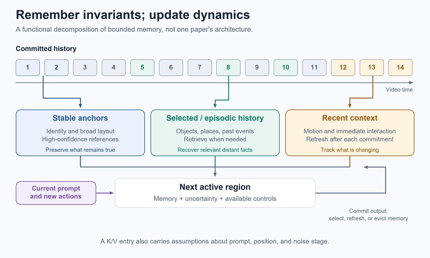
LongLive-RAG makes generated latent history content-addressable, helping the generator access nonlocal evidence beyond a recent window. Ring Forcing emphasizes object permanence together with memory capacity, using training that makes distant retrieval consequential for prediction.
These directions expose another important difference: memory availability is not memory use. A model can receive a distant frame and still ignore it if recent context already minimizes its loss. To learn retrieval, the training task must sometimes require information that the recent context cannot supply. Otherwise, an expensive memory bank may be functionally decorative.
7.8 KV Compression, Sparse Attention, and Cache-Oriented Forcing
This branch has expanded rapidly. Its methods belong in the same discussion because they change what historical evidence the deployed transition reads, how it is represented, or how much reading costs. They should still be distinguished from self-rollout training paradigms.
| Representative work | Dominant intervention | Question it clarifies |
|---|---|---|
| Deep Forcing | Training-free deep sinks and importance-based cache compression | Which persistent context supports fidelity without excessive repetition? |
| Relax Forcing | Structured sink, recent-tail, and selected historical roles | Does temporal placement matter more than raw memory size? |
| Light Forcing | Chunk-aware hierarchical sparse attention | How should compute be allocated across local and historical dependencies? |
| Sparse Forcing | Trainable persistent visual blocks and native sparse attention | Can memory retention and sparse computation be learned together? |
| Hybrid Forcing | Compact linear temporal state plus local block-sparse attention | Can evicted history contribute to a bounded recurrent summary? |
| Focused Forcing | Training-free selection varying by generated frame and attention head | Should all queries and heads receive the same history budget? |
| Future Forcing | Training-free cache decisions using a proxy for future query statistics | Can estimated later relevance improve retention beyond current attention scores? |
| Recency Forcing | Noise-stage-dependent attenuation of distant context, in training-free or trained modes | Can eventual eviction become less disruptive by reducing dependence beforehand? |
Two deductions follow. First, attention importance is conditional on the current query, noise stage, and positional representation. A token with low attention now may carry a fact needed later; an apparently important token may simply duplicate many others. Second, eviction is a modeling intervention. A network trained while all context remains available may behave poorly when that context disappears abruptly.
Recency-oriented attenuation and future-oriented retention are therefore not contradictory. They answer different questions: which dependencies should become weaker, and which evidence should remain available for later queries? A competent memory policy must negotiate both.
Compression and positional changes can also alter the features being read. A temporally shifted or merged K/V entry is not necessarily equivalent to re-encoding the corresponding clean video under its new context. The relevant test is continuation behavior after the policy is applied, not a nominal cache compression ratio alone.
7.9 From Long Video Generation to Persistent World State
The strongest interpretation of this route is a move from remembering images to remembering what those images imply. Identity should persist while pose changes. Object presence should persist through occlusion. Scene geometry should constrain later camera motion. A user edit should become part of the state rather than a transient visual effect.
Current cache mechanisms provide useful approximations, but a K/V cache is a set of neural representations, not an explicit inventory of objects, geometry, and event history. Long consistent samples alone do not establish a complete world model.
A more ambitious formulation would maintain a state $m_k$ that is updated after each commitment and tested under interventions that require old facts. The decisive experiments would involve leaving and revisiting locations, occluding and recovering objects, changing instructions, and preserving irreversible events over time.
This gives the route a clear destination: the generator should remain plastic in its dynamics while being selective about which facts it is allowed to forget. Longer context is one resource for that goal. Better state representation, retrieval supervision, and controlled forgetting are equally central.
Part IV — A Unified Perspective
The four routes describe different interventions, yet all operate on the same continuing generation process. A new schedule changes the states the model visits; a new memory policy changes the evidence available in those states; and a new supervisor changes which continuations are preferred. We can now bring these interactions together to build a taxonomy that explains both the relationships among forcing methods and the conditions under which their improvements should transfer.
8. A Unified Taxonomy of the Forcing Family
The taxonomy is most useful when it predicts what a change can and cannot fix. A method name is an entry point; the deployed transition is the object of analysis.
8.1 Four Mismatches, Four Technical Routes
| Mismatch | Dominant route | What must become aligned | What alignment alone leaves open |
|---|---|---|---|
| Architecture and information | Causal adaptation and information-compatible distillation | The target with the student’s observable inputs | The distribution of generated historical states |
| State distribution | Self-rollout or model-dependent history training | Training states with deployment states | Noise schedules, memory span, and the quality of supervision |
| Denoising trajectory | Heterogeneous-noise, rolling, and flexible schedules | Training configurations with active-window inference | Irrevocable historical errors and distant facts |
| Horizon and context | Long-rollout supervision, retrieval, and bounded memory | Retained evidence and supervision with long deployment | The accuracy and responsiveness of each transition |
The branches are not additive modules whose benefits can always be summed. A memory change alters state visitation. A rolling schedule alters what a causal initialization must support. A differentiable cache changes how future losses train earlier representations. A reward changes the desired output distribution even when the architecture remains fixed.
This is why the most plausible development path is iterative: make a coherent deployment procedure, identify its dominant failure, and adapt the corresponding part of learning. Independently assembling the best reported component from each branch may produce a combination that none of those components was trained to support.
8.2 What Is Actually Being “Forced”?
The term spans several distinct interventions. Teacher forcing specifies the conditioning history. Self forcing specifies how that history is generated. Diffusion and trajectory-oriented forcing specify uncertainty configurations. Causal distillation constrains the information compatibility of supervision. Context-oriented forcing changes the evidence available over long horizons. Reward and sample-based objectives change which output distribution should be preferred.
A more complete description of a system would therefore specify
\[\mathcal C=\left(\mathcal I,\ d_h,\ q_{\boldsymbol\lambda},\ \Pi,\ U,\ \mathcal L\right),\]where $\mathcal I$ is the permitted information, $d_h$ the history distribution, $q_{\boldsymbol\lambda}$ the training noise-configuration distribution, $\Pi$ the inference procedure, $U$ the memory-update policy, and $\mathcal L$ the supervising objective. This tuple is a descriptive framework, not a new forcing algorithm.
It makes otherwise ambiguous comparisons explicit. Two methods can use the same objective but different histories; the same history but different cache representations; or the same inference schedule but different supervisors. Saying that both are “DMD-based” or both are “self-forcing” leaves most of the important model specification unstated.
8.3 Training-Time Forcing and Inference-Time Intervention
A training intervention changes what the weights learn to do. An inference intervention changes the state or computation presented to those weights. Either can improve the stream, but they provide different evidence about the source of improvement.
A training-free cache policy that reduces drift suggests that the pretrained transition already contains useful competence which the original context presentation failed to access. A learned sparse-memory mechanism additionally adapts the transition to its new information pattern. Neither observation establishes that all retraining is unnecessary or that all cache policies require it.
The distinction also matters for composition. Applying a new cache policy to a self-rollout-trained model changes the loop that generated its training states. Mild changes may generalize well; aggressive ones may reopen the mismatch. Compatibility should be measured after the components are combined.
This is the practical meaning of a deployment contract: specify the chunks, noise stages, cached representations, positional rules, and control interface that the trained transition expects. The weights and that contract together define the streaming generator.
8.4 When “Forcing” Becomes a Naming Convention
The family is coherent as a research conversation, but it is not one mathematically closed class. Some names directly inherit the idea of forcing a training history. Others identify memory policies, attention kernels, reward objectives, or deployment infrastructure.
This naming breadth is harmless as long as it does not replace analysis. The useful test is to ask which variable a method changes and which mismatch that variable controls. A training-free cache method should not be credited with on-policy weight optimization. A flexible offline editing mode should not be counted as immediate streaming response. A representation-based objective should not be assumed to reproduce a teacher’s score field.
There is also a boundary to the conversion story. Native autoregressive training can address some mismatches before a bidirectional teacher is ever introduced. It remains relevant because it tells us which complications belong to streaming itself and which complications are artifacts of the chosen conversion pipeline.
8.5 A Diagnostic Framework for Evaluating New Claims
A useful evaluation should discriminate among failure mechanisms rather than collapse everything into one score. The following interventions are conceptual diagnostics; each requires matched settings and careful control of side effects.
| Suspected failure | Informative comparison | What the result would suggest |
|---|---|---|
| Information-incompatible initialization | Compare initializations with compatible causal targets at a matched student budget | An architectural or target contribution, provided training effort is controlled |
| Exposure to generated errors | Compare data-prefix continuation with free-running continuation using the same sampler | Sensitivity to self-generated histories |
| Unsupported denoising schedule | Change the schedule while controlling step budget, context, and attention access | Dependence on noise-state coverage or scheduling compatibility |
| Missing long-range evidence | Remove or restore distant relevant memory in a return or occlusion task | Whether memory is causally used for the tested dependency |
| Motion collapse disguised as consistency | Report motion and meaningful event progress alongside identity and image quality | Whether apparent stability is achieved by freezing behavior |
First-output latency, steady-state throughput, and action-to-visible-response latency should be reported separately. The last includes control ingestion, buffering, denoising, and decoding. A pipeline can be excellent at steady-state throughput while maintaining several stages of delayed response.
Quality should also be measured over time, with late-window scores and drift profiles rather than only pooled averages. Long-memory claims need tasks in which old evidence is necessary, not merely helpful. Robustness claims need control changes and meaningful motion, not only static prompts.
Finally, comparisons need a shared backbone, resolution, duration, chunk representation, step budget, precision, and hardware specification. The numerical improvements reported by the cited papers belong to their own evaluation setups. They are evidence for mechanisms, not a common leaderboard assembled by this article.
9. The Evolution of Streaming Video Generation
The evolution is best understood as several interacting changes in what the model is responsible for. It is not a single line in which every newer forcing method replaces every older one.
9.1 Clean History to Self-Generated History
The first change moves responsibility from producing a plausible local continuation to producing a continuation that remains usable inside feedback. This makes rollout state visitation part of training design.
The more mature interpretation retains clean-history supervision where it is informative. It does not demand that every stage use the final inference distribution from the beginning. Reliable initialization, controlled model-dependent corruption, and free-running refinement can play different roles in a curriculum.
The next frontier is representative state coverage under realistic control changes and memory operations. A model trained on its own static-prompt short rollouts is still only aligned with that restricted deployment. “Self-generated” is a provenance statement, not a guarantee of sufficient coverage.
9.2 Bidirectional Teacher to Causal Teacher
The second change makes the transfer target information-compatible. Its enduring lesson is to identify the mathematical object being transferred: conditional denoising, a noise-to-endpoint mapping, a joint output distribution, or a preference over outputs.
A causal teacher is especially useful for paired causal trajectory transfer. A bidirectional teacher can remain valuable as a judge of generated clips. Real videos can provide supervision outside a fixed teacher’s preferred modes. Reward models can reshape those preferences, at the cost of introducing their own blind spots.
The direction is therefore toward task-appropriate supervisors, rather than a requirement that one teacher architecture serve every stage. A good training design may use several kinds of evidence while leaving the inference generator compact.
9.3 Strict AR to Rolling Joint Denoising
The third change treats local revision as a resource. Strict autoregression minimizes lookahead and offers a simple dependency graph. Rolling generation spends a bounded future buffer to preserve local cooperation. Flexible generation can adapt this choice to an operating regime.
There is no universal best point. Immediate action response, offline cinematographic coherence, single-GPU efficiency, and distributed pipeline utilization place different values on the same buffer. Evaluation should specify which constraints define the operating point.
This suggests an important systems principle: measure how much unfinished future the model maintains, not just how many completed past frames it reads. Both affect resources, but only the former directly describes the amount of speculative work that may need revision after an unexpected control update.
9.4 Short Context to Persistent Memory
The fourth change moves from retaining recent imagery to preserving facts at different timescales. It requires deliberate memory writing, retrieval, updating, and forgetting.
The September LongLive-Plug explores a related scaling question: distilling reusable capabilities, including long-context error correction, into adapters transferable to compatible downstream models. This shifts attention from repeating a full conversion for every specialization to separating reusable streaming competence from task-specific conditioning.
The compatibility condition is essential. Memory correction learned under one backbone and context interface is not automatically portable to arbitrary representations. Persistent competence is easiest to reuse when the state representation and deployment contract remain recognizable.
9.5 Few-Step Video to Interactive Generation
Interactive generation requires an entire path from input to visible response. Few-step sampling is one component. Control adaptation, cache refresh, scheduling, communication, and streaming VAE decoding can dominate the remaining delay.
minWM makes this full conversion pipeline explicit for camera-controllable models, joining controllable adaptation with causal training and few-step distillation. Next Forcing expands causal training supervision to multiple future chunks, illustrating that a representation can be trained for longer predictive usefulness without observing unknown future actions.
Infrastructure also changes which learning setups are feasible. LongLive-2.0 combines parallel training, low-precision execution, and streaming decoding, and reports a direct long autoregressive tuning route with subsequent acceleration adapters. These advances challenge the assumption that a particular multi-stage distillation pipeline is the only practical route to streaming.
The publicly released Wave Forcing project emphasizes a block-causal mixed-noise frontier and distributed stage pipelining. At this article’s cutoff, its repository provides inference code and a preview checkpoint while listing the paper and training code as forthcoming. Its systems results should accordingly be distinguished from a fully documented training study.
The common implication is that inference efficiency emerges from compatible computation and state transitions. Counting denoising evaluations alone cannot describe it.
9.6 Streaming Video to World Models
Streaming video supplies a useful substrate for world modeling because it permits sequential observations and interventions. But a visually coherent stream is insufficient evidence of a reliable simulator. The model must respond consistently to actions, retain hidden state, and preserve consequences across returns and occlusions.
An instructive boundary case is Mutual Forcing, a native autoregressive audio-video framework in which shared few-step and multi-step modes provide complementary self-distillation and generated-history training. It lies beyond the central bidirectional-DiT conversion setting, but shows that information alignment and state alignment can be designed into a causal model from the outset.
For broader world models, the important question is whether the retained state supports the interventions a user or agent will actually make. A generated room that looks plausible after a camera turn is useful. A room that preserves an object placed there minutes earlier is a stronger capability. Neither automatically establishes correct dynamics outside the tested distribution.
The forcing framework helps formulate these requirements precisely. It does not by itself supply explicit geometry, physical correctness, or causal identification. Those remain additional modeling and evaluation problems.
10. Conclusion
Converting a bidirectional video DiT into a streaming generator changes the meaning of a successful prediction. A chunk must be plausible under restricted information, robust to a past the model helped create, compatible with the active denoising schedule, and useful to a future that will depend on a compressed record of it.
The four routes expose four responsibilities: choose observable targets, train on representative states, support the intended uncertainty trajectory, and preserve the evidence needed over time. Their interactions explain why causal distillation, self-rollout, flexible denoising, and memory engineering should be analyzed together while retaining their conceptual differences.
The deepest shift in the forcing family is from optimizing a model that completes clips to optimizing a model that inhabits a continuing process. Its quality depends on the state it visits and the state it leaves behind. The enduring measure of progress is how well that process preserves competence as decisions become irreversible, controls change, and the past grows beyond the model’s immediate view.
11. References
The entries below link to primary papers or official project materials. Years refer to the first public preprint where applicable; conference versions can appear later. The text uses these works as evidence for the conceptual analysis rather than as directly comparable benchmark entries.
- Chen et al. (2024). Diffusion Forcing: Next-token Prediction Meets Full-Sequence Diffusion.
- Yin et al. (2024). From Slow Bidirectional to Fast Autoregressive Video Diffusion Models — CausVid.
- Song et al. (2025). History-Guided Video Diffusion — DFoT and History Guidance.
- Huang et al. (2025). Self Forcing: Bridging the Train-Test Gap in Autoregressive Video Diffusion.
- Yang et al. (2025). LongLive: Real-time Interactive Long Video Generation.
- Liu et al. (2025). Rolling Forcing: Autoregressive Long Video Diffusion in Real Time.
- Cui et al. (2025). Self-Forcing++: Towards Minute-Scale High-Quality Video Generation.
- Lu et al. (2025). Reward Forcing: Efficient Streaming Video Generation with Rewarded Distribution Matching Distillation.
- Yi et al. (2025). Deep Forcing: Training-Free Long Video Generation with Deep Sink and Participative Compression.
- Guo et al. (2025). End-to-End Training for Autoregressive Video Diffusion via Self-Resampling — Resampling Forcing.
- Zhang et al. (2026). Reward-Forcing: Autoregressive Video Generation with Reward Feedback.
- Zhu et al. (2026). Causal Forcing: Autoregressive Diffusion Distillation Done Right for High-Quality Real-Time Interactive Video Generation.
- Lv et al. (2026). Light Forcing: Accelerating Autoregressive Video Diffusion via Sparse Attention.
- Chen et al. (2026). Context Forcing: Consistent Autoregressive Video Generation with Long Context.
- Zhao et al. (2026). Relax Forcing: Relaxed KV-Memory for Consistent Long Video Generation.
- Li et al. (2026). Long-Horizon Streaming Video Generation via Hybrid Attention with Decoupled Distillation — Hybrid Forcing.
- Xu et al. (2026). Sparse Forcing: Native Trainable Sparse Attention for Real-time Autoregressive Diffusion Video Generation.
- Zhou et al. (2026). Mutual Forcing: Dual-Mode Self-Evolution for Fast Autoregressive Audio-Video Character Generation.
- Zhao et al. (2026). Causal Forcing++: Scalable Few-Step Autoregressive Diffusion Distillation for Real-Time Interactive Video Generation.
- Cai et al. (2026). Focused Forcing: Content-Aware Per-Frame KV Selection for Efficient Autoregressive Video Diffusion.
- Chen et al. (2026). LongLive-2.0: An NVFP4 Parallel Infrastructure for Long Video Generation.
- Luo et al. (2026). Future Forcing: Future-aware Training-free KV Cache Policy for Autoregressive Video Generation.
- Zhao et al. (2026). minWM: A Full-Stack Open-Source Framework for Real-Time Interactive Video World Models.
- Hu et al. (2026). LongLive-RAG: A General Retrieval-Augmented Framework for Long Video Generation.
- Xu et al. (2026). Next Forcing: Causal World Modeling with Multi-Chunk Prediction.
- Zheng et al. (2026). Causal-rCM: A Unified Teacher-Forcing and Self-Forcing Open Recipe for Autoregressive Diffusion Distillation in Streaming Video Generation and Interactive World Models.
- Ma et al. (2026). Flex-Forcing: Towards a Unified Autoregressive and Bidirectional Video Diffusion Model.
- Li et al. (2026). Ms. Forcing: Efficient Streaming Video Generation with Multi-Scale Patchification and Attention.
- Zhu et al. (2026). Stream Forcing: Constructing Unified Training Trajectory for Robust Streaming Video Generation.
- Xue et al. (2026). Ring Forcing: Towards Precise Long-Term Memory for Autoregressive Video Diffusion.
- Cao et al. (2026). Recency Forcing: Bridging the Long-Horizon Gap in Autoregressive Video Generation.
- Zhang et al. (2026). From Scores to Samples: Elastic Forcing for Autoregressive Video Generation.
- Wang et al. (2026). Self-Aligned Forcing: Streaming Video Diffusion with Differentiable Noisy History.
- Yang et al. (2026). LongLive-Plug: Once-for-All Distillation for Video Generation.
- Park et al. (2026). LongTake: Learning to Sustain Dynamics in Long-Horizon Video Generation.
- Lin et al. (2026). Enhancing Autoregressive Video Generation via Representation Adversarial Distillation — Radian.
- DENG Lab MLSys Team (2026). Wave Forcing — official inference repository and release status. Project release; a public paper is listed as forthcoming at the cutoff.