Controllable Video Generation
📅 Published:
📘 TABLE OF CONTENTS
- 1. Images and Keyframes Controls
- 2. Spatial and Structural Controls
- 3. Motion and Trajectory Controls
- 4. Camera Controls
- Reference
The graphs in this article are generated with the aid of GPT-Image-2 and Nano-Banana-2.
Controllable video generation extends text-to-video and image-to-video models with explicit control over visual states, spatial structure, motion, and camera trajectories. This article introduces the main control types, including keyframes, poses, depth maps, masks, trajectories, optical flow, reference videos, and camera parameters. It organizes their implementations around condition construction, spatiotemporal encoding, and feature injection, while comparing soft conditioning with hard latent constraints. The goal is to provide a unified understanding of how controllable video systems balance control accuracy, temporal coherence, appearance preservation, and compatibility with pretrained video generation models.
1. Images and Keyframes Controls
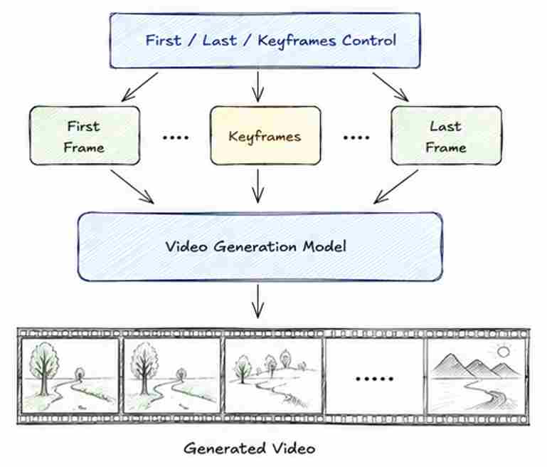
Image and keyframe controls constrain a generated video with one or more visually specified states. Instead of describing the entire sequence only through text, the user provides an image at a known timestamp, such as the first frame, the last frame, or several intermediate keyframes. The model must preserve the important visual content of these frames while generating plausible motion and temporally coherent transitions between them.
These controls reduce temporal ambiguity. First-frame conditioning anchors the initial subject, composition, and appearance. Last-frame conditioning specifies a target state that the generated sequence should reach. First-and-last-frame control turns generation into a transition problem between two visual endpoints, while multiple keyframes provide sparse visual milestones for storyboard-based generation, animation planning, and interactive video creation.
A key distinction is whether the supplied frames are treated as soft conditions or hard constraints. A soft condition guides the model toward the reference image but does not guarantee that the generated frame exactly matches it. A hard constraint directly fixes the corresponding latent or pixel frame during sampling. The implementation routes discussed below differ mainly in where the keyframe information enters the generator and how strongly it constrains the final output.
1.1 Application Scenarios of Image and Frame Controls
Image and Frame Controls are widely used in many scenarios, including but not limited to:
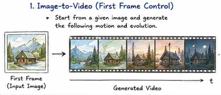
- Single-Frame Control for Image-to-Video Generation: The most common single-frame setting is first-frame control, where the generation starts from a given input image and the model produces the subsequent video content.
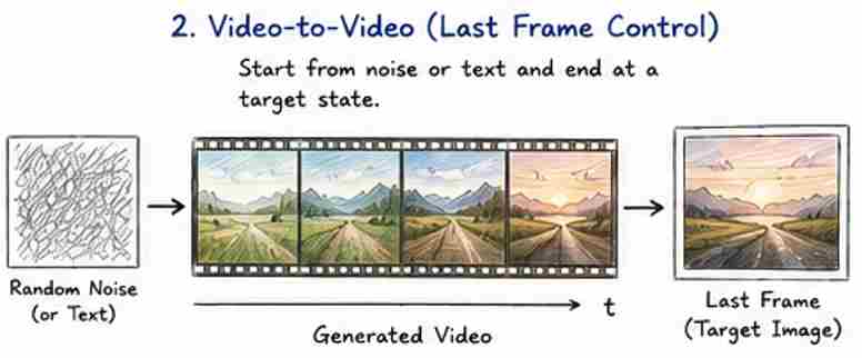
- End-Frame Control for Target-Driven Video Generation: A less common but conceptually important setting is last-frame control, where the user specifies the desired target image and asks the model to generate a sequence that reaches that state.
- Two-Frame Control for Start-and-End Constrained Generation: A stronger multi-frame setting is start-and-end frame control, where both the first frame and the last frame are specified.
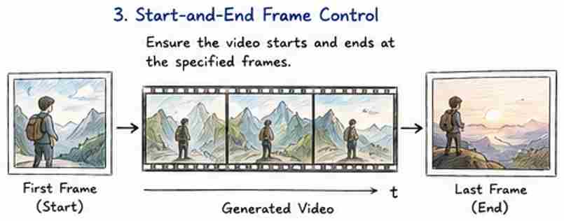
- Multi-Frame Control for Storyboard and Narrative Planning: When multiple sparse frames are provided at selected timestamps, the model can perform storyboard-to-video generation. Each frame functions as a key visual beat in the narrative, and the model generates the in-between content to create a continuous sequence. This is highly useful in previsualization, filmmaking, animation planning, and content design workflows, where creators often know the important shots but do not want to manually create every frame. In this context, frame control acts as a bridge between high-level visual planning and full video synthesis.

- Interactive and User-Guided Video Creation: Finally, frame control provides a natural interface for interactive generation, where users iteratively add, modify, or refine frames during the generation process. A user may begin with a single image, then later provide a target ending frame, and later insert additional keyframes to refine the motion or narrative. This makes image and frame controls especially suitable for human-in-the-loop creative systems, because they allow users to gradually shape the video without requiring dense low-level control. In practice, this supports iterative editing, controllable creative workflows, and real-time or streaming video generation.

1.2 Problem Formulation
We consider the problem of extending a pretrained image-to-video model to support an arbitrary combination of first-frame, last-frame, and intermediate-keyframe conditions.
Let the target video contain \(T\) pixel-space frames:
\[x_0 = [x_0^{(0)},x_0^{(1)},\ldots,x_0^{(T-1)}] \in \mathbb{R}^{B\times 3\times T\times H\times W}.\]The superscript denotes the physical video-frame index, while the subscript $0$ denotes clean data in diffusion or flow-matching notation. Assume that the user provides a set of keyframes:
\[\mathcal{K} = \left\{ \left(k_1,I_{k_1}\right), \left(k_2,I_{k_2}\right), \ldots, \left(k_K,I_{k_K}\right) \right\}\]where:
- \(k_i\in\{0,\ldots,T-1\}\) is the desired pixel-frame position;
- \(I_{k_i}\in\mathbb{R}^{3\times H\times W}\) is the corresponding keyframe image.
The set may contain arbitrary subsets during training and inference. The desired conditional distribution is:
\[p_\theta \left( x_0 \mid \{I_k\}_{k\in\mathcal K}, \mathcal K, c_{\text{text}} \right),\]where \(c_{\text{text}}\) denotes an optional text prompt. Three main implementation patterns can be distinguished:
- Route A: keyframes as additional conditional latents.
- Route B: keyframes inserted into the generative latent state.
- Route C: keyframes represented as external visual-token memory.
The routes are not mutually exclusive. Practical systems often combine low-level latent conditions with high-level visual tokens.
1.3 Route A: Sparse Conditional Latents with Temporal Alignment
Route A represents the supplied keyframes as a sparse conditional video aligned with the original pixel-space timeline. The sparse video is encoded by the same video VAE used by the base model, and the resulting conditional latent is provided as an additional input to the Video DiT.
Sparse Conditional Video Construction: A sparse conditional video is constructed as:
\[x_{\text{cond}}^{(t)} = \begin{cases} I_t, & t\in\mathcal K,\\[10pt] 0, & t\notin\mathcal K. \end{cases}\]Thus,
\[x_{\text{cond}} \in \mathbb{R}^{B\times3\times T\times H\times W}.\]We can visualize sparse conditional video construction through the following figure:
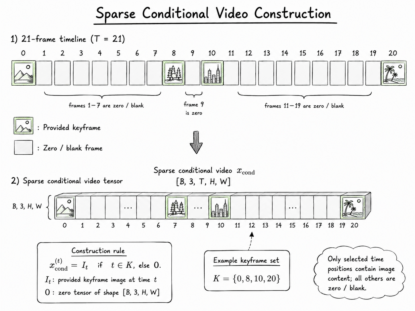
The zero-filled frames are placeholders used to preserve the full video tensor shape. They do not mean that the model should generate black frames. The sparse video is encoded by a pretrained video VAE:
\[z_{\text{cond}} = E_{\text{3D-VAE}}(x_{\text{cond}}) \in \mathbb{R}^{B\times C\times T_z\times H'\times W'}.\]Because a video VAE contains temporal convolutions and temporal downsampling, one latent frame may summarize several neighboring pixel frames. The temporal interaction depends on the VAE architecture. In a causal VAE, earlier keyframes may influence later latent positions, while future keyframes do not propagate backward into earlier positions.
The conditional latent is therefore aligned with the compressed video timeline, but it is not necessarily aligned one-to-one with individual pixel frames.
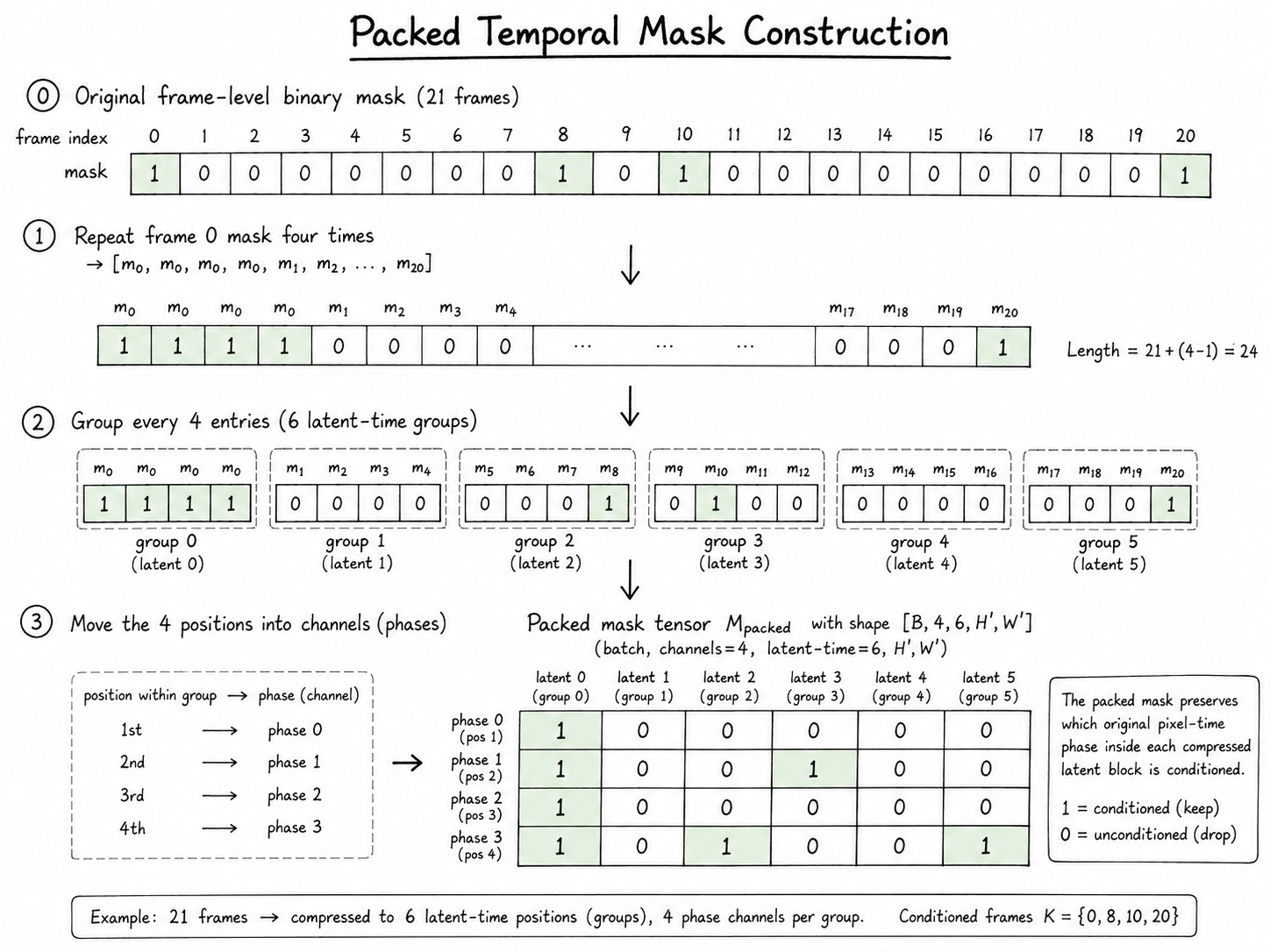
Pack Temporal Mask Construction: A binary frame mask specifies which pixel-space frames contain valid conditions:
\[m^{(t)} = \begin{cases} 1, & t\in\mathcal K,\\[10pt] 0, & t\notin\mathcal K. \end{cases}\]For the 21-frame example, the mask tells the DiT that frames $0$, $8$, $10$, and $20$ were explicitly supplied. Suppose the 3D VAE uses a Wan-style temporal compression rule, the packed temporal mask is:
\[M_{\text{packed}} = \begin{bmatrix} 1&0&0&0&0&0\\[10pt] 1&0&0&1&0&0\\[10pt] 1&0&0&0&0&0\\[10pt] 1&0&1&0&0&1 \end{bmatrix}.\]This transformation is parameter-free. It is best understood as temporal phase packing, analogous to moving fine-resolution temporal indices into channels.
Channel-Wise Conditional Injection: Supposed The target clean video is encoded by 3D VAE from pixel to latent spaces is:
\[z_0 = E_{\text{3D-VAE}}(x_0).\]At diffusion or flow-matching time $s$, the target latent is perturbed:
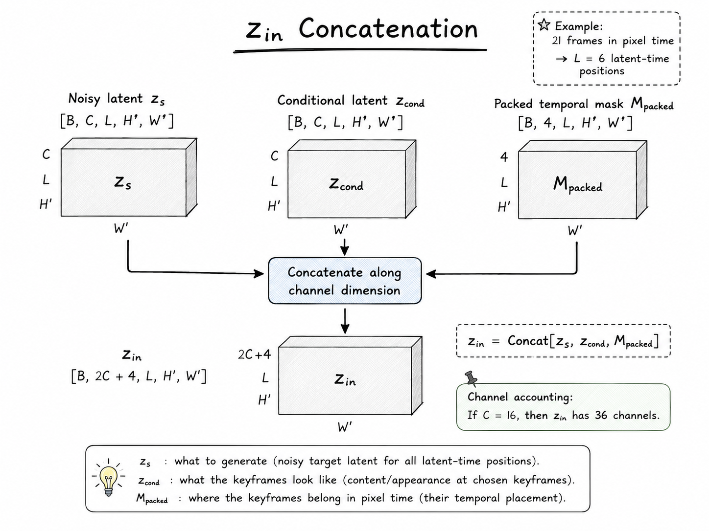
\[z_s = \alpha_s z_0 + \sigma_s\epsilon, \qquad \epsilon\sim\mathcal N(0,I).\]The Video DiT input is then constructed by channel-wise concatenation:
\[z_{\text{in}} = \operatorname{Concat} \left[ z_s,\, z_{\text{cond}},\, M_{\text{packed}} \right].\]where:
\[z_s \in \mathbb{R}^{B\times C\times T_z\times H'\times W'}, \\[10pt] z_{\text{cond}} \in \mathbb{R}^{B\times C\times T_z\times H'\times W'}, \\[10pt] M_{\text{packed}} \in \mathbb{R}^{B\times r_t\times T_z\times H'\times W'}.\]The complete input is:
\[z_{\text{in}} \in \mathbb{R}^{B\times(2C+r_t)\times T_z\times H'\times W'}.\]For $C=16$ and \(r_t=4\):
\[z_{\text{in}} \in \mathbb{R}^{B\times36\times6\times H'\times W'}.\]This input-level concatenation is the defining condition-injection mechanism of Route A. The conditional latent carries what the keyframes look like, while the mask specifies where in physical video time those keyframes belong.
1.3.1 Training and Constraint Strength
Arbitrary-keyframe generation requires arbitrary-keyframe training. For each training video, the keyframe set should be sampled from different positions and with different cardinalities:
\[\mathcal T_{\mathrm{key}} \sim p_{\mathrm{keyframe}}.\]Training only with first-frame conditions does not automatically produce a model that understands arbitrary intermediate or last-frame conditions.
Condition dropout is also useful. The image conditions, text condition, or individual keyframes can be randomly removed so that one model can support different combinations of text-to-video, image-to-video, and multi-keyframe generation.
Route A provides a soft constraint. The model receives the keyframes as conditions, but the generated latent at a conditioned timestamp is not explicitly replaced with the supplied keyframe latent. Therefore,
\[\hat x_0^{(k)} \approx I_k\]may hold approximately, but exact equality is not guaranteed.
1.4 Route B: Temporal Latent Inpainting with Frame Replacement
Route B treats keyframe control as temporal latent inpainting. Instead of adding a separate conditional latent branch, it directly inserts the clean latent representations of the supplied keyframes into the corresponding positions of the noisy video latent.
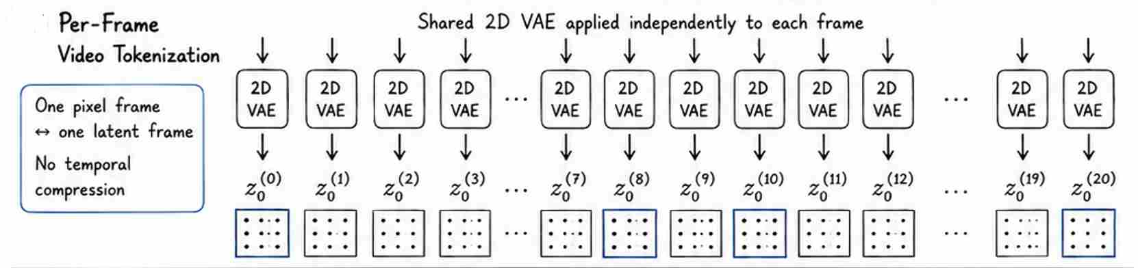
This route requires a tokenizer that preserves identifiable temporal positions. The simplest implementation applies a shared image VAE independently to every frame:
\[z_0^{(t)} = E_{\mathrm{2D\text{-}VAE}} (x_0^{(t)}),\]producing
\[z_0 = [z_0^{(0)},z_0^{(1)},\ldots,z_0^{(T-1)}] \in \mathbb{R}^{B\times C\times T\times H_z\times W_z}.\]Here,
\[T_z=T,\]so each pixel-space frame corresponds to one latent frame. More generally, Route B requires a temporally preserving tokenizer, not necessarily a 2D VAE, as long as the conditioned frames can be independently identified and replaced.
Mixed Clean-Noisy Latent: A binary temporal mask indicates the conditioned positions:
\[M^{(t)} = \begin{cases} 1, & t\in\mathcal T_{\mathrm{key}},\\[10pt] 0, & t\notin\mathcal T_{\mathrm{key}}. \end{cases}\]The mask can be represented as
\[M \in \{0,1\}^{B\times1\times T\times1\times1}.\]The complete target video latent is first perturbed:
\[z_s = \alpha_s z_0 + \sigma_s\epsilon.\]
Each supplied keyframe is separately encoded as
\[z_{\mathrm{key}}^{(k)} = E(I_k), \qquad k\in\mathcal T_{\mathrm{key}}.\]During training, the keyframes are sampled from the ground-truth video, so
\[z_{\mathrm{key}}^{(k)} = z_0^{(k)}.\]The noisy latent is then replaced at conditioned positions:
\[\widetilde z_s = M\odot z_{\mathrm{key}} + (1-M)\odot z_s.\]The resulting sequence contains clean latent frames at the known positions and noisy latent frames at the unknown positions.
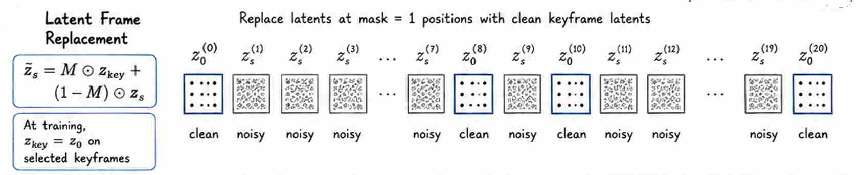
The model should also receive the validity mask, either as an additional input channel, a token-type embedding, or a per-frame timestep indicator:
\[v_\theta = v_\theta (\widetilde z_s,s,M,c_{\mathrm{text}}).\]Without an explicit indicator, an arbitrary-keyframe model may not reliably distinguish clean condition frames from noisy generation frames.
1.4.1 Masked Training Objective
Because the conditioned frames are already supplied, the denoising or flow-matching loss is normally applied only to the unknown positions:
\[\mathcal L = \left\| (1-M)\odot \left[ v_\theta (\widetilde z_s,s,M,c) - v^\star \right] \right\|_2^2.\]The model learns to reconstruct the missing temporal regions while using the clean keyframes as boundary or intermediate conditions.
1.4.2 Iterative Clamping During Sampling
The replacement operation must be repeated at every solver step. Suppose the current sampling state is (z_{s_i}). Before evaluating the model, the known positions are restored:
\[\widetilde z_{s_i} = M\odot z_{\mathrm{key}} + (1-M)\odot z_{s_i}.\]The model predicts the denoising direction:
\[v_i = v_\theta (\widetilde z_{s_i},s_i,M,c),\]and the solver updates the unknown region:
\[z_{s_{i+1}} = \operatorname{SolverStep} (z_{s_i},v_i).\]Before the next model evaluation, the keyframe positions are clamped again. If this replacement is performed only once at initialization, later solver updates can modify the known frames and the constraint will gradually disappear.
Route B therefore provides a much stronger constraint than Routes A and C. At the latent level, it can maintain
\[\hat z_0^{(k)} = z_{\mathrm{key}}^{(k)}.\]However, VAE reconstruction is not perfectly lossless:
\[D(E(I_k)) \approx I_k.\]Latent replacement therefore does not guarantee pixel-level identity. When exact pixel preservation is required, the decoded frame may be replaced with the original image after generation, although this can introduce small discontinuities around the keyframe timestamp.
1.5 Route C: Timestamped Keyframe Memory with Cross-Attention
Route C represents every supplied keyframe as an independent set of visual tokens rather than placing it directly into the temporally compressed video latent grid. Each keyframe is processed by an image encoder, augmented with an explicit video timestamp and optional frame-type embedding, and stored in an external keyframe memory. The noisy video tokens query this memory through cross-attention during every Video DiT block or a selected subset of blocks.
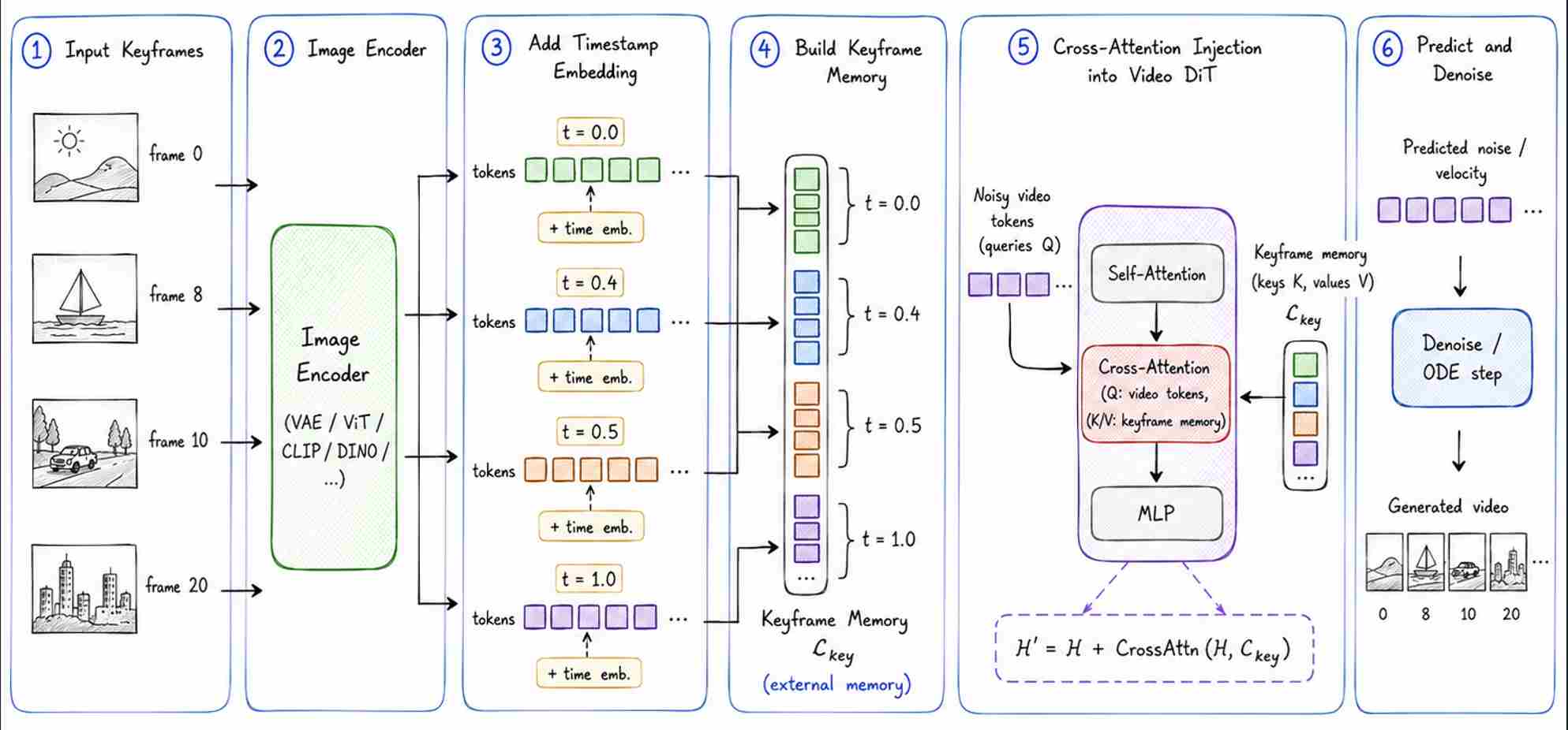
Independent Keyframe Encoding: Each keyframe is processed by an image encoder:
\[F_k = E_{\mathrm{img}}(I_k) \in \mathbb{R}^{B\times N_I\times D_I}.\]A learned projection maps the features into the Video DiT hidden dimension:
\[E_k = F_kW_{\mathrm{proj}} \in \mathbb{R}^{B\times N_I\times D}.\]For spatially precise keyframe control, the encoder should retain patch-level or multiscale spatial tokens. A global pooled embedding may preserve semantics or identity but usually discards the detailed layout needed to reproduce a keyframe accurately.
Different encoders preserve different information. CLIP and SigLIP features are strong for semantic alignment, DINO-style features often preserve useful local correspondences, while VAE or reconstruction-oriented features retain more color, texture, and spatial detail. A practical model may combine several feature types.
Timestamp Embedding: Each keyframe is assigned a normalized timestamp:
\[\tau_k = \frac{k}{T-1}.\]The timestamp is mapped into an embedding:
\[e_k^{\mathrm{time}} = E_{\mathrm{time}}(\tau_k) \in \mathbb{R}^{D}.\]It is added to every visual token from that keyframe:
\[\widetilde E_k = E_k + e_k^{\mathrm{time}}.\]All keyframe-token sets are concatenated into a shared memory:
\[C_{\mathrm{key}} = [ \widetilde E_{k_1}; \widetilde E_{k_2}; \ldots; \widetilde E_{k_K} ] \in \mathbb{R}^{B\times KN_I\times D}.\]A padding mask is required when samples contain different numbers of keyframes.
Cross-Attention-Based Keyframe Injection: At a Video DiT layer, video tokens query the keyframe memory:
\[Q_l = H_lW_Q, \qquad K_{\mathrm{key}} = C_{\mathrm{key}}W_K, \qquad V_{\mathrm{key}} = C_{\mathrm{key}}W_V.\]The basic attention update is
\[H_l' = H_l + g_l \operatorname{CrossAttn} (H_l,C_{\mathrm{key}}),\]where (g_l) is an optional learned gate. Initializing (g_l) near zero allows the newly added condition branch to preserve the pretrained model behavior at the start of post-training.
Timestamp embeddings on the keyframe tokens are necessary but not sufficient for reliable temporal placement. The video query tokens must also carry their own temporal positions. A stronger attention formulation explicitly models the relative temporal distance between a video token at time (t) and a keyframe at time (k):
\[A_{t,k} = \operatorname{Softmax}_k \left( \frac{ Q_tK_k^\top }{ \sqrt d } + b(t,k) \right),\]where (b(t,k)) is a learned or predefined temporal bias.
Temporal routing can further restrict which keyframes are available to each output interval. For a target time between two keyframes,
\[k_a<t<k_b,\]the video token may primarily attend to the surrounding pair
\[{I_{k_a},I_{k_b}},\]rather than all keyframes in the sequence. Such routing reduces temporal leakage and prevents unrelated keyframes from being mixed.
1.5.1 Constraint Strength
Route C is a soft conditioning mechanism. Cross-attention makes the keyframe information available to the generator, but it does not force the output latent at time (k) to equal the encoded keyframe latent:
\[\hat x_0^{(k)} \not\equiv I_k.\]It is effective for semantic consistency, identity preservation, appearance transfer, and flexible multi-reference conditioning, but it may be insufficient for exact spatial or pixel-level reproduction.
For stronger keyframe fidelity, Route C is often combined with Route A or Route B. The visual-token memory supplies semantic and identity information, while latent concatenation or replacement preserves lower-level spatial details.
A related variation places the keyframe tokens and video tokens in one unified sequence and uses self-attention:
\[S = [ S_{\mathrm{video}}; S_{\mathrm{keyframe}} ].\]This allows bidirectional interaction between keyframe and video tokens, whereas standard cross-attention treats the keyframes as an external memory. The two designs differ in computational cost and in how strongly the modalities are coupled.
2. Spatial and Structural Controls
Text prompts are effective at describing semantic content—what objects should appear, what style the video should have, or what action should occur—but they are poor interfaces for specifying exact geometry. A prompt such as “a dancer moves across a stage” does not determine the dancer’s joint locations, trajectory, scale, camera perspective, foreground mask, or scene depth at every frame.
Spatial-structure-controlled video generation addresses this limitation by conditioning a video diffusion or flow model on explicit structural signals such as pose sequences, depth maps, edge maps, segmentation masks, optical flow, bounding boxes, trajectories, surface normals, or camera-ray maps.
2.1 Application Scenarios of Image and Frame Controls
There are many different forms of spatial condition control signals, as well as many different application scenarios.
Human pose: Pose-controlled generation is used for character animation, dance transfer, virtual humans, digital fashion, and reenactment. Animate Anyone, for example, separates appearance preservation through a ReferenceNet from motion control through a pose guider and temporal modeling.
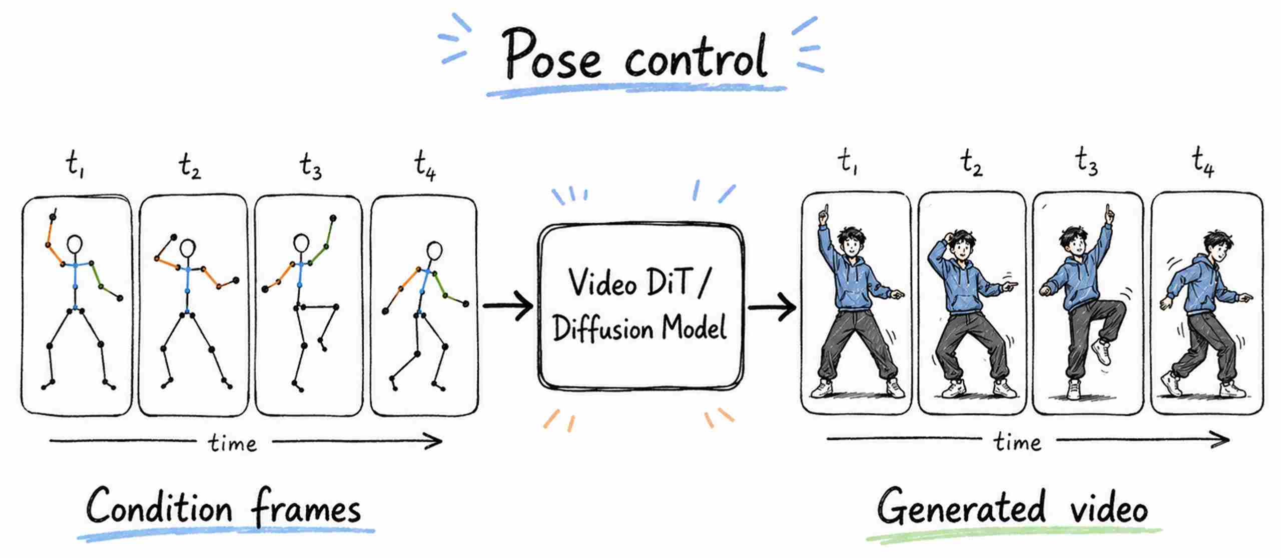 Figure 14: Human pose Control
Edge and sketch sequences: Edge conditions offer stronger shape constraints than text while leaving color, texture, lighting, and material unspecified.
SketchVideo supports sketch control on only one or two arbitrary keyframes and propagates those sparse conditions to other frames through inter-frame attention. Its control blocks predict residual features for the Video DiT rather than requiring a complete copy of the backbone.
 Figure 15: Edge and sketch Control
Depth maps: Depth is more geometry-aware than an edge map because two visually adjacent regions can be assigned very different distances.
 Figure 16: Depth maps Control
Optical flow and motion fields: Optical flow directly represents image-plane motion:
\[F_t \in \mathbb{R}^{2\times H\times W}.\]The first channel describes horizontal displacement and the second vertical displacement. Flow control is particularly useful when appearance should remain flexible but motion should follow a source video or hand-designed deformation field.
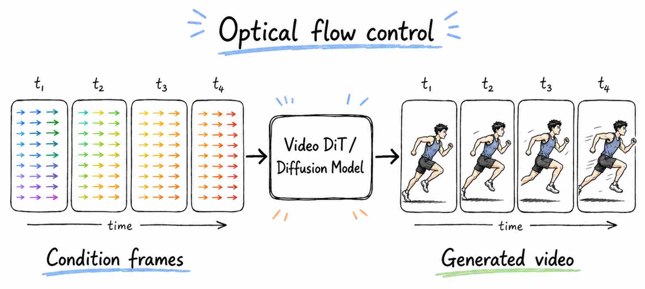 Figure 17: Optical flow and motion fields Control
Masks and semantic segmentation: A mask can play two different roles: a structural condition, where its silhouette guides generated content; a hard editing constraint, where unmasked latent regions are repeatedly restored from the source video.
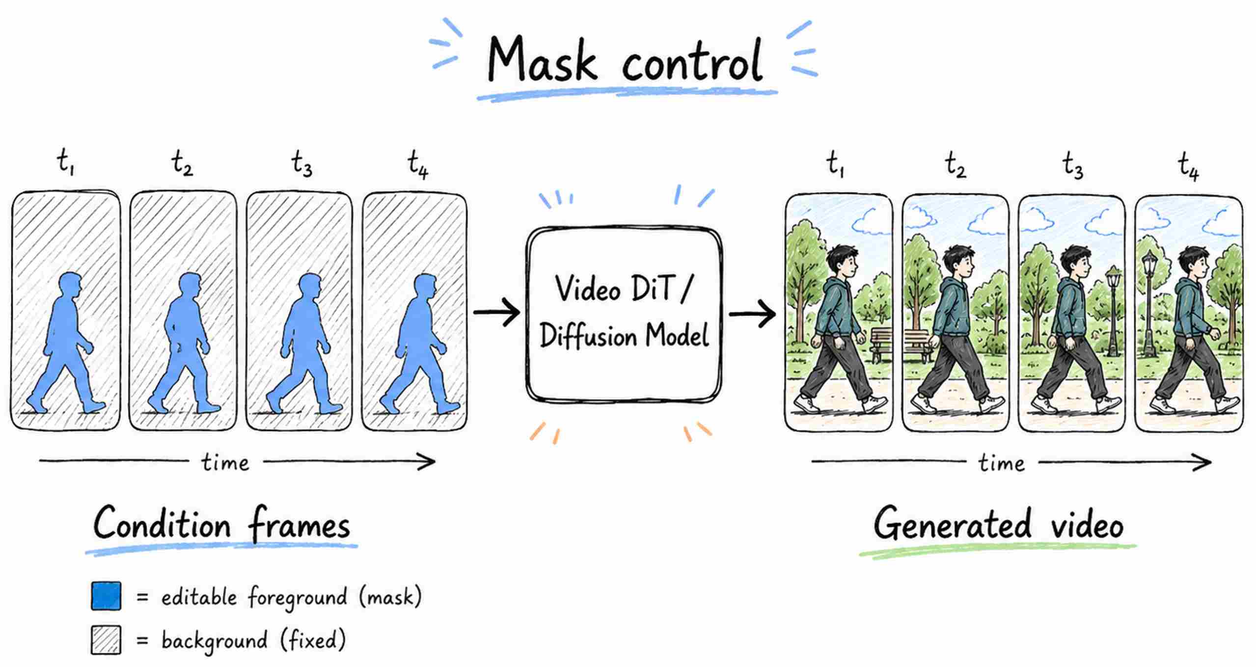 Figure 18: Masks and semantic segmentation Control
2.2 Main Implementation Strategies
Spatially controlled video generation can be organized into three stages: condition organization, spatiotemporal condition encoding, and condition injection. The first stage determines how sparse or dense user inputs cover the target timeline. The second converts those inputs into position-sensitive features aligned with the video latent. The third determines how strongly and where those features affect the Video DiT.
2.2.1. Condition Organization
Let the target video contain $T$ frames:
\[X=\{X_1,\ldots,X_T\}.\]A structural condition may be available for every frame, only a few keyframes, or a single frame. Regardless of the input form, the final objective is to provide the generator with control information over the complete latent timeline.
When every frame has a corresponding pose, edge, depth, mask, or flow map, which also known as dense control, the conditions naturally form a control video:
\[C={C_1,\ldots,C_T} \in \mathbb{R}^{B\times C_c\times T\times H\times W}.\]Each condition frame directly constrains the corresponding output frame:
\[C_t \leftrightarrow X_t.\]No temporal completion is required; the main task is to encode the control video while preserving its frame-wise spatial structure.
When conditions are available only at several keyframes,
\[\mathcal K={t_1,\ldots,t_K}, \qquad K<T,\]the missing control information must be propagated to the uncontrolled frames. One option is to explicitly reconstruct a dense condition sequence before generation. This is practical for low-dimensional continuous controls such as bounding boxes, point trajectories, camera poses, or skeletal joint coordinates. For example, a trajectory can be interpolated as
\[p_t=(1-\rho)p_{t_a}+\rho p_{t_b}, \qquad \rho=\frac{t-t_a}{t_b-t_a}.\]Direct interpolation is much less reliable for rasterized pose maps, edges, masks, or depth maps because it can produce double contours, blurred masks, incorrect occlusions, and unrealistic deformation. For these conditions, a more general strategy is to encode only the valid keyframes and propagate their features through inter-frame attention, temporal transformers, feature warping, or learned motion modules. The model therefore constructs a dense feature sequence without necessarily generating a complete pixel-space condition video.
A single condition image requires the same distinction. If it represents a time-invariant constraint, such as a fixed background mask or static scene layout, it can be broadcast across the timeline:
\[C_t=C^\star,\qquad t=1,\ldots,T.\]If it represents a condition at one particular time, such as the initial pose or a sketch at frame (t_k), it should be treated as a keyframe constraint. Its temporal position must be provided explicitly, and its influence should be propagated rather than blindly repeated.
A validity mask is commonly used to distinguish missing conditions from genuine zero-valued inputs:
\[m_t= \begin{cases} 1,&t\in\mathcal K,\\[10pt] 0,&t\notin\mathcal K. \end{cases}\]The condition-processing module therefore receives both the sparse sequence and its availability mask. Conceptually, this stage transforms heterogeneous user input into control information covering the complete target timeline.
2.2.2 Spatiotemporal Condition Encoding
After organization, the condition must be mapped from pixel or parameter space to a representation compatible with the video latent. Suppose the video VAE produces
\[z_\tau \in \mathbb{R}^{B\times C_z\times T'\times H'\times W'}.\]The condition encoder should produce a correspondingly aligned feature tensor:
\[F_c = \mathcal E_c(C,m) \in \mathbb{R}^{B\times C_f\times T'\times H'\times W'}.\]The central requirement is not merely to recognize the semantic content of the condition. It is to preserve the correspondence
\[(t,h,w) \longleftrightarrow (t',h',w'),\]so that a pose joint, object boundary, depth value, or mask region at a particular time and location can affect the corresponding video token.
The encoder may use 3D convolutions, per-frame 2D convolutions followed by temporal attention, tubelet embeddings with a video transformer, or multiscale spatiotemporal blocks. Dense conditions can be processed directly as a control video. Sparse conditions usually require an additional propagation module that converts keyframe features into a full sequence:
\[\widetilde F_t = \mathcal P \left( {F_{t_k},t_k}_{k=1}^{K},t \right).\]For attention-based propagation, a target-frame feature can query the available keyframes:
\[a_{t,k} = \operatorname{softmax}_k \left( \frac{q_t^\top k_{t_k}}{\sqrt d} + b(t,t_k) \right),\] \[\widetilde F_t = \sum_{k=1}^{K}a_{t,k}v_{t_k}.\]The temporal bias \(b(t,t_k)\) encodes frame distance, while the content-dependent attention weights allow nonlinear motion and different spatial regions to reference different keyframes.
A generic video-understanding encoder should not be used unchanged for this purpose. Classification and retrieval models commonly compress a clip into a global representation:
\[z_{\mathrm{video}} \in \mathbb{R}^{B\times D}.\]Such a representation may identify that the video contains “a running person,” but it usually discards the exact frame, position, boundary, and local motion information required for spatial control. A video-understanding backbone can still provide initialization, but global pooling should be removed, dense patch or tubelet tokens should be retained, and the model should be adapted for position-sensitive control encoding.
The output of this stage is therefore not merely a semantic video embedding, but a dense spatiotemporal control representation aligned with the generator.
2.2.3 Condition Feature Injection
Once the aligned condition features have been obtained, they must be integrated into the Video DiT. The main designs differ in where the control enters the network and how much authority it has over the pretrained generator.
The most direct approach is input-channel concatenation:
\[z_{\mathrm{in}} = \operatorname{Concat}_{\mathrm{channel}} [z*\tau,F_c].\]The combined tensor is then patchified and processed by the DiT. This provides strong low-level control because the condition is visible from the first layer, but it changes the input projection and becomes less convenient when many control modalities are added.
A more modular strategy uses a side branch or lightweight adapter. The condition pathway produces residuals for selected DiT layers:
\[R_l=\mathcal C_l(F_c),\]and then
\[\widetilde H_l = H_l+\lambda_lP_l(R_l).\]Here, \(P_l\) maps the control feature to the hidden dimension, and \(\lambda_l\) controls its strength. A full ControlNet-style branch provides strong multilevel control but increases memory and parameter cost. A smaller adapter is more efficient, although it may provide weaker control for difficult structural constraints.
Cross-attention treats video tokens as queries and condition tokens as keys and values:
\[Q=H_lW_Q, \qquad K=F_cW_K, \qquad V=F_cW_V,\]and
\[\widetilde H_l = H_l+ \operatorname{softmax} \left( \frac{QK^\top}{\sqrt d} \right)V.\]Global cross-attention is flexible but may weaken strict spatial correspondence. For pose, depth, edge, and mask control, aligned or local attention is often preferable, allowing a video token to attend mainly to the corresponding time-space location or a nearby region.
Condition features may also modulate normalized hidden states:
\[(\gamma_l,\beta_l)=g_l(F_c,\tau),\]and
\[\widetilde H_l = \gamma_l\odot\operatorname{LN}(H_l)+\beta_l.\]Global modulation is efficient and suitable for coarse motion or semantic attributes. Precise structural control requires token-wise modulation so that different times and spatial positions receive different parameters.
These mechanisms are complementary rather than mutually exclusive. A practical system may concatenate coarse condition features at the input, inject multiscale residuals through adapters, and use aligned cross-attention for sparse keyframe propagation.
The quality of spatial control ultimately depends on all three stages: the condition must cover the intended timeline, the encoder must preserve explicit time-space correspondence, and the injection mechanism must provide sufficient control without destroying the pretrained video prior.
3. Motion and Trajectory Controls
Text prompts describe what should happen in a video, but they usually provide weak control over where an object moves, how fast it moves, which region should deform, or whether a new character should follow a specific action. Trajectory-controlled video generation addresses this limitation by introducing explicit motion conditions alongside the source appearance and text description.
The motion condition may be sparse, such as a few user-drawn point trajectories, or dense, such as a full optical-flow field. It may describe only object displacement, or additionally constrain scale, shape, local deformation, pose, and temporal dynamics. The general objective is to combine an appearance source with a time-aligned motion representation:
\[\text{appearance}+\text{motion condition} \longrightarrow \text{controlled video}.\]A useful system should preserve the identity and visual details of the source content while following the specified motion smoothly. It must also infer the unobserved consequences of the control, including object deformation, occlusion, background revelation, depth changes, and interactions between controlled and uncontrolled regions.
3.1 Application Scenarios of Motion and Trajectory Controls
Single-point and multi-point trajectories provide the most lightweight form of motion control. A user can click on an object and drag the selected point along a desired path. A single point is often sufficient for controlling approximate object translation, such as moving a car along a road or dragging a product across an advertisement. Multiple points provide stronger constraints because they can describe different parts of the same object. For example, trajectories attached to the front, rear, and center of a car can implicitly specify translation, rotation, and scale changes more accurately than a single center trajectory.
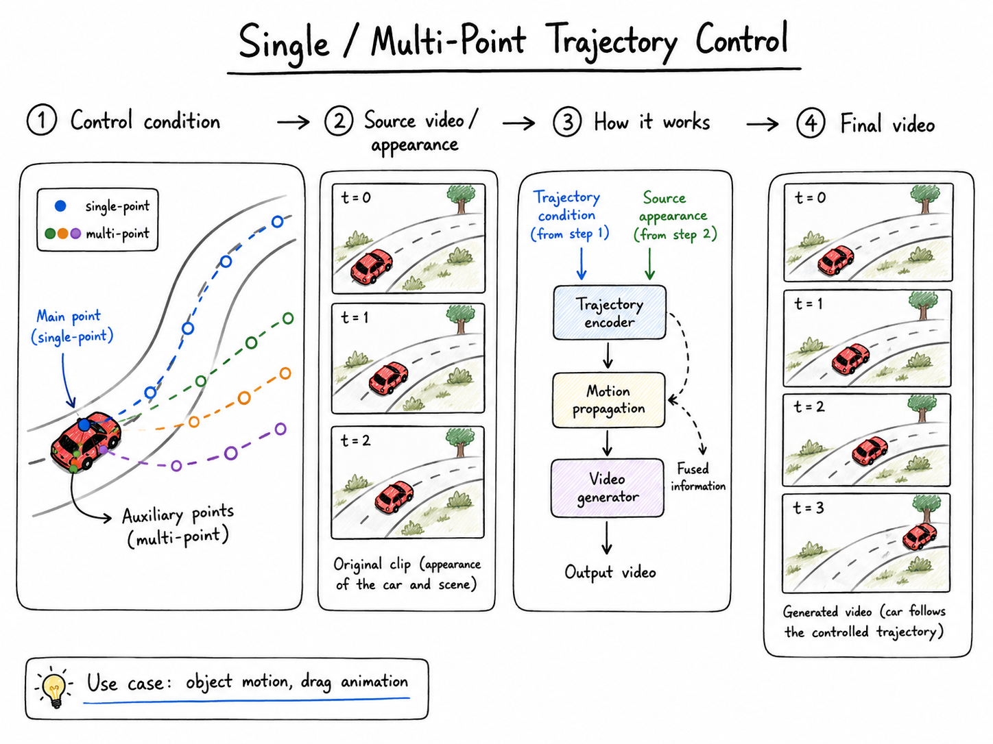
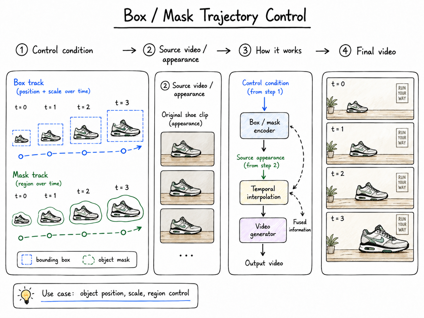
Box and mask trajectories control the spatial extent of an object over time. A box sequence specifies the object position and approximate scale in each frame, making it suitable for product placement, object animation, multi-object layout control, and approach-or-retreat motion. A mask sequence provides finer region-level constraints and can represent changing silhouettes, partial deformation, or irregular object boundaries. These controls are useful when the desired motion cannot be adequately represented by only a few tracked points.
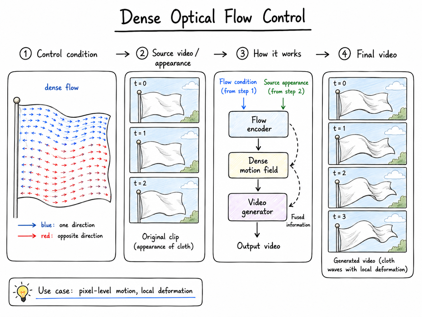
Dense optical flow provides pixel-level motion supervision. Instead of describing only a small set of locations, it assigns a displacement vector to every spatial position. This makes it suitable for cloth waving, hair movement, water flow, facial deformation, smoke, vegetation motion, and other non-rigid dynamics. Dense flow can also represent different motion directions inside the same object, which is difficult to express using a single trajectory or bounding box.
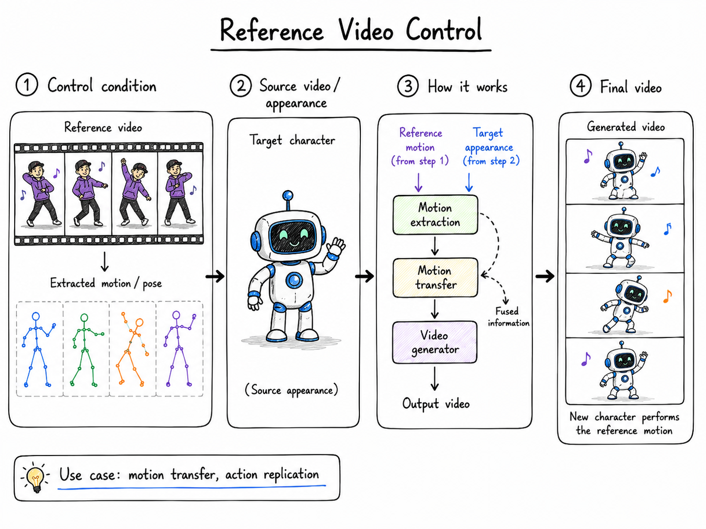
Reference-video control transfers motion from an existing video to new visual content. A human dance video may drive a stylized character, a camera movement may be reused in another scene, or the motion pattern of one object may be applied to another. In this setting, the user does not manually define trajectories. Instead, the system extracts motion representations such as poses, point tracks, optical flow, camera motion, or learned motion tokens from the reference video and combines them with the target appearance.
3.2 Rasterizing Coordinates into Spatiotemporal Condition Maps
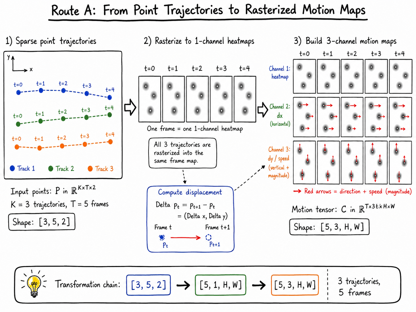
A point trajectory is commonly represented as a sequence of image-space coordinates:
\[P={(x_t,y_t)}_{t=0}^{T-1}.\]For multiple tracks, the condition becomes:
\[P\in\mathbb{R}^{K\times T\times 2},\]where \(K\) is the number of controlled points. Visibility flags, object identifiers, motion confidence, or temporal masks may be added when points disappear because of occlusion.
We converts sparse point coordinates into spatially aligned condition maps. For $K$ trajectories over $T$ frames, the input is
\[P\in\mathbb{R}^{K\times T\times2}, \qquad p_{k,t}=(x_{k,t},y_{k,t}).\]Each point is rasterized as a Gaussian heatmap:
\[H_{k,t}(u,v) = \exp\left( -\frac{(u-x_{k,t})^2+(v-y_{k,t})^2}{2\sigma^2} \right).\]Multiple trajectories can be stored in separate channels or merged into one frame-level map:
\[H_t(u,v)=\sum_{k=1}^{K}H_{k,t}(u,v).\]The coordinates are therefore transformed into a sparse condition video:
\[P\in\mathbb{R}^{K\times T\times2} \longrightarrow H\in\mathbb{R}^{T\times1\times H\times W}.\]To encode motion direction and speed explicitly, the displacement between consecutive points is computed as
\[\Delta p_{k,t} = p_{k,t+1}-p_{k,t} = (\Delta x_{k,t},\Delta y_{k,t}).\]The horizontal and vertical components are written around the corresponding trajectory locations:
\[D_t^x(u,v) = \sum_{k=1}^{K} H_{k,t}(u,v)\Delta x_{k,t},\] \[D_t^y(u,v) = \sum_{k=1}^{K} H_{k,t}(u,v)\Delta y_{k,t}.\]The final rasterized motion condition is
\[C_t= \left[ H_t,, D_t^x,, D_t^y \right], \qquad C\in\mathbb{R}^{T\times3\times H\times W}.\]The heatmap specifies where the controlled points should appear, while the displacement channels specify how they move.
A spatiotemporal encoder then projects these maps into latent-aligned motion features:
\[F_{\mathrm{traj}} = E_{\mathrm{traj}}(C), \qquad F_{\mathrm{traj}} \in \mathbb{R}^{B\times D\times T_z\times H_z\times W_z}.\]These features can be injected into a video UNet or DiT through input concatenation, residual control branches, cross-attention, or feature modulation.
However, trajectory maps alone describe only the motion of sparse spatial anchors. They do not explicitly tell the model which complete object the anchors belong to. An object mask can address this ambiguity through two different mechanisms.
3.2.1 Implicit Entity Feature Propagation
The first mechanism uses the mask to extract an object-level identity feature from the source frame. Let
\[F_0\in\mathbb{R}^{D\times h\times w}\]be the first-frame feature map and
\[M_{\mathrm{obj}}\in{0,1}^{h\times w}\]be the object mask. A masked pooling operation produces an entity embedding:
\[e_{\mathrm{obj}} = \frac{ \sum_{u,v} M_{\mathrm{obj}}(u,v)F_0(u,v) }{ \sum_{u,v}M_{\mathrm{obj}}(u,v) }.\]This feature summarizes the complete object rather than only the local appearance around the dragged point. It is then placed at each trajectory location:
\[E_t(u,v) = H_t(u,v)e_{\mathrm{obj}}.\]The resulting condition contains both the target location and the identity of the controlled object. Through convolutions, spatial attention, and temporal attention, the video generator learns to propagate this entity-aware motion cue from the local anchor to the complete object.
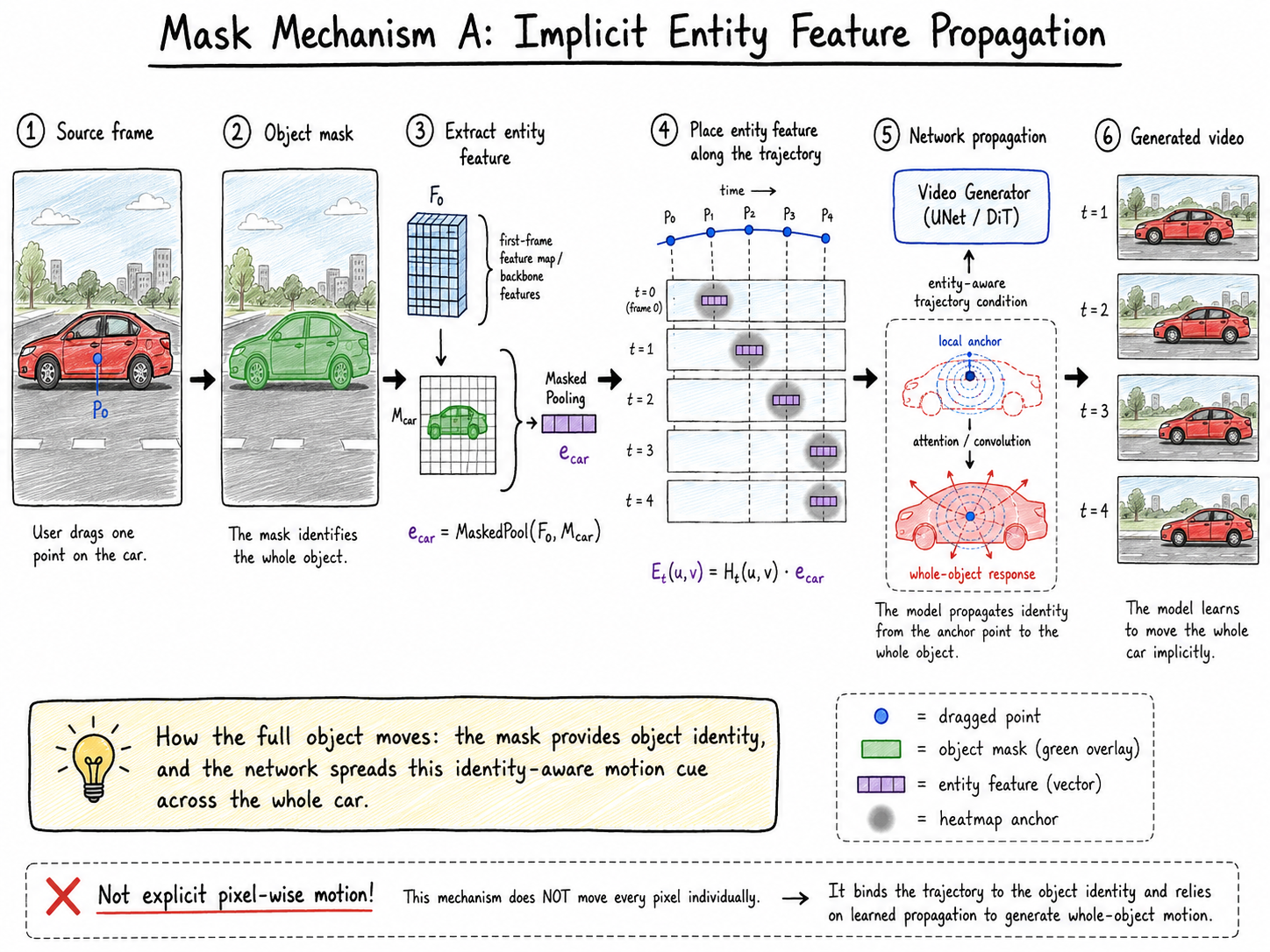
Whole-object motion is therefore produced implicitly by the learned video prior. It supports natural deformation and appearance synthesis, but the motion constraint is relatively soft and may become unreliable for large displacements or precise geometric transformations.
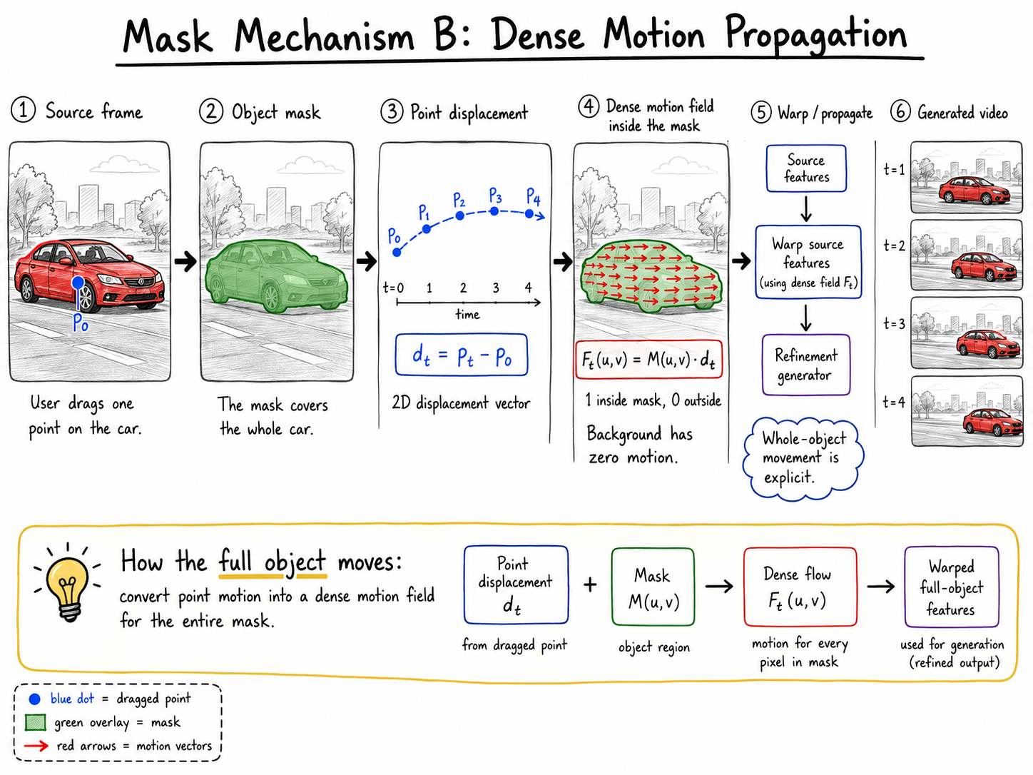
3.2.2 Explicit Dense Motion Propagation
The second mechanism uses the mask to expand point displacement into a dense motion field over the complete object region. For a single trajectory, the displacement from the initial point to frame (t) is
\[d_t=p_t-p_0.\]Under a rigid-translation assumption, every pixel inside the object mask receives the same displacement:
\[F_t(u,v) = M_{\mathrm{obj}}(u,v)d_t, \qquad F_t\in\mathbb{R}^{2\times H\times W}.\]Thus, \(F_t(u,v)=d_t\) inside the object and \(F_t(u,v)=0\) in the background. The sparse point motion has now become an explicit dense flow field describing where every object pixel should move.
The source appearance features can be warped using this field:
\[\widetilde F_t = \operatorname{Warp}(F_0,F_t).\]The warped features provide an initial estimate of the complete object at its target position. A video generator then refines the result, repairs boundaries, fills disoccluded background regions, and synthesizes changes such as wheel rotation, perspective variation, or local deformation.
With multiple trajectories, the motion field need not be a uniform translation. The relative movement of several points can be used to estimate an affine, piecewise-affine, thin-plate-spline, or learned non-rigid transformation:
\[\lef\{ p_{k,0}\rightarrow p_{k,t} \right\}_{k=1}^{K} \longrightarrow F_t(u,v).\]This allows different parts of the object to receive different motion vectors, making multi-point control suitable for rotation, scaling, articulated motion, and local deformation.
The two mask mechanisms therefore solve complementary problems. Implicit entity propagation uses the mask to determine which object is moving and relies on the generator to spread the motion cue across that object. Dense motion propagation uses the mask to determine which spatial region receives motion and explicitly assigns a displacement to every location inside it:
\[\text{entity binding} \quad\text{vs.}\quad \text{pixel-wise motion propagation}.\]In practice, they can also be combined: entity features preserve object identity, dense motion fields provide stronger geometric control, and the generative model produces a realistic temporally consistent video.
3.3 Box and Mask Trajectories
A box trajectory can be written as:
\[B_t=(c_x^t,c_y^t,w_t,h_t),\]where the center controls position and the width and height control scale. Rotation angles or object identities may also be included. A mask trajectory is usually represented as:
\[M\in{0,1}^{T\times H\times W}.\]Boxes are typically rasterized into binary box maps, soft spatial heatmaps, or coordinate-based embeddings. Masks can be directly processed as a condition video. When the user provides only a few key boxes or masks, the system must first construct intermediate conditions. Box centers and sizes can often be interpolated numerically, but mask interpolation is more difficult because object shape, visibility, and topology may change over time. Learned mask propagation, video segmentation, object tracking, or feature-space correspondence is therefore generally more reliable than direct pixel interpolation.
The box or mask encoder extracts temporally aligned region features, which are fused with source appearance features. The source object may be represented by cropped image embeddings, masked visual tokens, or multiscale features from the first frame. Object identifiers are important in multi-object scenes so that each trajectory remains associated with the correct entity.
Box conditions provide strong layout constraints but weak shape information. Masks offer more precise region control but require more annotation and more robust temporal propagation. In both cases, the video generator must synthesize the content revealed when an object moves away, maintain object identity, and produce realistic changes in perspective and occlusion.
3.4 Dense Optical Flow
Dense optical flow represents motion between adjacent frames as:
\[F_t(x,y)= \bigl(\Delta x_t(x,y),\Delta y_t(x,y)\bigr).\]A sequence of flow fields provides a dense, time-dependent motion condition over the complete video. The flow may come from a reference clip, a flow-estimation model, a physical simulator, or a learned completion network that converts sparse user controls into dense motion.
The flow condition is usually encoded by a convolutional network or a spatiotemporal video encoder. Because the condition is already spatially dense, it can be aligned directly with the video latent grid after spatial and temporal downsampling. The resulting features may be injected into the denoiser at multiple resolutions.
Flow can also be used operationally rather than only as an encoded condition. Source image or latent features can be warped according to the predicted flow:
\[\widetilde{f}_{t+1} = \operatorname{Warp}(f_t,F_t).\]The warped features provide an explicit estimate of where visual content should move. A generative model then refines these features, fills disoccluded regions, corrects flow errors, and synthesizes appearance changes that cannot be explained by two-dimensional warping alone.
Dense flow enables detailed local motion but does not fully represent three-dimensional geometry. Large viewpoint changes, newly visible surfaces, occlusion, and motion along the depth axis remain ambiguous. For this reason, optical-flow control is often combined with depth, segmentation, source appearance, or learned video priors.
3.5 Reference-Video Control
Reference-video control separates motion from appearance. A motion encoder processes the reference clip and extracts a transferable representation, while an appearance encoder processes the target character or target scene:
\[m_{\mathrm{ref}}=E_{\mathrm{motion}}(V_{\mathrm{ref}}), \qquad a_{\mathrm{target}}=E_{\mathrm{appearance}}(I_{\mathrm{target}}).\]The extracted motion may be represented explicitly as human pose, facial landmarks, point trajectories, optical flow, object masks, or camera poses. Explicit representations provide interpretable control and are suitable for structured domains such as human animation. Learned motion tokens are more general but may entangle motion with the reference subject’s appearance, background, or identity.
During generation, the motion representation is temporally aligned with the target video and injected into the video model. Pose maps and flow fields are commonly processed through residual control branches. Motion tokens may enter through cross-attention, while target appearance features provide identity and texture information through separate attention or feature-injection pathways.
The major challenge is motion–appearance disentanglement. The output should reproduce the reference dynamics without copying the reference person, clothing, background, or visual style. Differences in body proportions and topology must also be handled. For example, directly transferring human joint coordinates to a robot may cause unrealistic limb motion unless the system adapts the reference motion to the target structure. Retargeting modules, normalized pose representations, correspondence learning, and target-aware motion adaptation are therefore often required.
4. Camera Controls
Camera trajectory control aims to determine how the virtual camera moves while a video is being generated. Unlike object trajectory control, which specifies how an entity moves inside the scene, camera control changes the viewpoint from which the entire scene is observed. Even when every object is static, moving the camera changes the projected position, scale, visibility, and appearance of almost every region in the video.
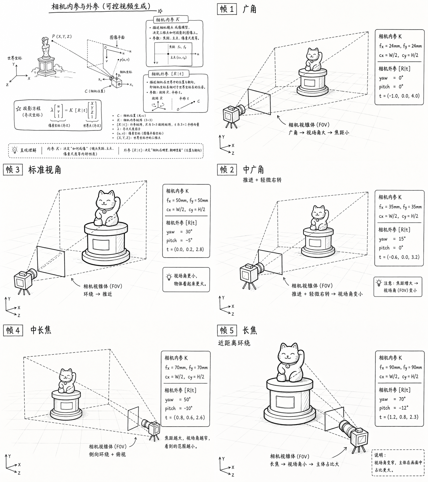
This makes camera motion a special form of video control. A lateral camera translation produces depth-dependent parallax: nearby objects move faster across the image than distant backgrounds. Camera rotation changes the viewing direction of the whole frame. A forward dolly enlarges objects according to their depth and reveals new occlusion relationships, while an orbit exposes previously invisible surfaces of the subject. Changing focal length affects the field of view without necessarily changing the camera position.
A pretrained video generator may already reproduce pans, dolly shots, tracking shots, and orbiting views because such motion appears naturally in its training videos. However, this capability is usually implicit. Given only a text prompt or a first frame, the model may choose an arbitrary camera motion. Camera-controlled post-training therefore introduces an explicit interface that maps a user-specified camera trajectory to the corresponding visual transformation.
4.1 Camera Conditions
A camera trajectory is usually represented by a sequence of camera intrinsics and extrinsics:
\[\mathcal{C} = \left\{ K_t, R_t, t_t \right\}_{t=0}^{T-1}.\]The intrinsic matrix
\[K_t= \begin{bmatrix} f_x^t & 0 & c_x^t\\[5pt] 0 & f_y^t & c_y^t\\[5pt] 0 & 0 & 1 \end{bmatrix}\]describes how the camera forms an image. The focal lengths \((f_x^t,f_y^t)\) determine the field of view, while \((c_x^t,c_y^t)\) specifies the principal point. In many systems, the intrinsics are fixed throughout the video and only the extrinsics change. More flexible systems also support zooming, focal-length variation, principal-point shifts, or lens distortion.
The extrinsics describe the position and orientation of the camera. Under a world-to-camera convention,
\[X_t^c = R_t X^w + t_t,\]where \(R_t\) rotates a point from world coordinates into the camera coordinate system and \(t_t\) completes the coordinate transformation. The camera center in world coordinates is
\[o_t=-R_t^\top t_t.\]In practice, users rarely provide these matrices manually. They may select predefined motions such as pan, tilt, dolly, orbit, crane, or tracking shots; edit several camera key poses; import a trajectory from Blender or Unreal Engine; or estimate a trajectory from a reference video. These interfaces are eventually converted into a frame-by-frame sequence of \(K_t,R_t,t_t\).
4.2 From Global Camera Parameters to a Spatial Camera Condition
Although \(K_t,R_t,t_t\) completely define the camera, directly broadcasting the same camera vector to every spatial token is usually not the most effective representation. The camera parameters are global, while a video diffusion model processes a dense spatiotemporal grid. Different image locations correspond to different viewing directions, even within the same frame.
The mainstream solution is therefore to convert the frame-level camera parameters into a spatially aligned camera-ray field.
For a pixel or latent-grid position ((u,v)), the viewing direction in the camera coordinate system is
\[d_{t,u,v}^{c} = \operatorname{normalize} \left( K_t^{-1} \begin{bmatrix} u\v\1 \end{bmatrix} \right).\]It is then rotated into world coordinates:
\[d_{t,u,v}^{w} = R_t^\top d_{t,u,v}^{c}.\]Together with the camera center \(o_t\), this defines a ray
\[r_{t,u,v}(s) = o_t+s,d_{t,u,v}^{w}.\]A widely used representation is the Plücker ray embedding:
\[p_{t,u,v} = \left( d_{t,u,v}^{w}, ; o_t\times d_{t,u,v}^{w} \right) \in\mathbb{R}^{6}.\]The first three components describe where the ray points. The last three describe where the corresponding three-dimensional line lies relative to the world origin. Stacking all rays produces
\[P_{\mathrm{cam}} \in \mathbb{R}^{T\times H\times W\times 6}.\]This tensor can be interpreted as a camera-condition video, although it is not an RGB video. Each spatial location stores the geometry of the viewing ray associated with that frame and position. The conversion does not add new information beyond (K,R,t); it transforms global camera parameters into a representation that is naturally aligned with the spatial tokens of the video generator.
Before ray construction, the camera poses are normally expressed relative to the first frame:
\[T_t^{\mathrm{rel}} = T_0^{-1}T_t.\]This removes the arbitrary world coordinate system and makes the first camera pose the reference pose. Coordinate conventions must also be standardized, including world-to-camera versus camera-to-world matrices, axis directions, handedness, translation scale, image resizing, and cropping. When the input resolution changes, the intrinsic matrix must be updated accordingly.
4.3 Alignment with the Video Latent Grid
A video generator usually operates in a compressed latent space. Given an RGB video
\[x\in\mathbb{R}^{B\times3\times T_x\times H_x\times W_x},\]a video VAE produces
\[z\in\mathbb{R}^{B\times C_z\times T_z\times H_z\times W_z}.\]The camera condition must be aligned with this latent grid. One option is to construct a high-resolution ray field at the RGB resolution and use a camera encoder to downsample it. Another option is to sample the camera trajectory at the latent timestamps and construct rays directly on the \(H_z\times W_z\) latent grid.
For a DiT with spatial and temporal patchification, the camera condition is further converted into camera tokens:
\[P_{\mathrm{cam}} \rightarrow C_{\mathrm{cam}} \in \mathbb{R}^{B\times N\times D},\]where
\[N=T_pH_pW_p.\]Each camera token then corresponds to the same spatiotemporal region as one video token.
Temporal alignment is especially important for video VAEs that compress multiple RGB frames into one latent frame. The camera pose associated with a latent frame may be taken from the temporal center of its receptive field or obtained by interpolation over the corresponding RGB-frame poses.
4.4 Camera Condition Encoding
The ray field is usually processed by a dedicated camera encoder:
\[\left\{ F_{\mathrm{cam}}^{(l)} \right\}_{l=1}^{L} = E_{\mathrm{cam}} \left( P_{\mathrm{cam}} \right).\]A typical encoder begins with a linear projection, convolution, or patch embedding that maps the six-dimensional ray representation into a higher-dimensional feature space. Spatial blocks capture the arrangement of rays within each frame, while temporal attention or temporal convolution captures how the viewing geometry changes along the camera trajectory.
For a U-Net-style video generator, the encoder often produces multi-scale features:
\[F_{\mathrm{cam}}^{(l)} \in \mathbb{R}^{B\times C_l\times T_l\times H_l\times W_l}.\]Each feature map is matched to one resolution level of the video U-Net. For a DiT, the camera encoder may instead output a sequence of camera tokens with the same hidden dimension as the video tokens.
The camera encoder should primarily model viewing geometry rather than scene appearance. For this reason, many designs feed only ray or pose information into the camera branch and keep the pretrained video backbone frozen or mostly frozen. This reduces the risk that the camera module memorizes the visual style of the camera-labelled training set.
4.5 Injecting Camera Features into the Video Generator
The encoded camera condition must modify the denoising or flow-prediction network without destroying the pretrained model’s visual quality. The most common strategy is residual injection. At layer (l), the camera branch predicts a feature residual:
\[\Delta h_l^{\mathrm{cam}} = A_l \left( F_{\mathrm{cam}}^{(l)} \right),\]which is added to the main hidden state:
\[h_l' = h_l+ \Delta h_l^{\mathrm{cam}}.\]The output projection of the camera branch is often zero-initialized. At the beginning of training,
\[\Delta h_l^{\mathrm{cam}}\approx0,\]so the model behaves like the original pretrained generator. The camera branch then gradually learns how to steer the existing video-generation features.
Another common design uses cross-attention:
\[h_l' = h_l+ \operatorname{CrossAttn} \left( Q=h_l, K=C_{\mathrm{cam}}, V=C_{\mathrm{cam}} \right).\]This allows each video token to retrieve the camera geometry associated with the relevant frame and spatial position. Camera features may also generate adaptive normalization parameters:
\[(\gamma_l,\beta_l) = g_l(C_{\mathrm{cam}}),\] \[h_l' = (1+\gamma_l)\odot\operatorname{Norm}(h_l)+\beta_l.\]In U-Net video diffusion models, camera features are frequently injected into temporal or spatiotemporal blocks because camera motion primarily determines relationships between frames. In video DiTs, camera adapters may be inserted into selected self-attention blocks, cross-attention blocks, or geometry-sensitive middle layers. Injecting the condition into every layer is not always beneficial, because excessive camera conditioning may interfere with semantic generation, texture synthesis, or object identity.
A ControlNet-like side branch is also common. The branch processes the camera condition separately and produces zero-initialized residuals for multiple backbone layers:
\[h_l^{\mathrm{main}} \leftarrow h_l^{\mathrm{main}} + Z_l \left( h_l^{\mathrm{cam}} \right).\]This provides stronger structural control while preserving the pretrained backbone.
4.6 Training
Camera-control training requires videos paired with estimated or known camera trajectories:
\[\mathcal{D}_{\mathrm{cam}} = \left\{ x_i, y_i, \mathcal{C}*i \right\}_{i=1}^{N},\]where \(x_i\) is the video, \(y_i\) is the text or image condition, and \(\mathcal{C}_i\) contains the corresponding intrinsics and extrinsics. Camera poses can be recovered from real videos using structure-from-motion, visual odometry, or SLAM, while synthetic data can provide exact camera parameters.
The underlying diffusion or flow-matching objective does not need to change. For flow matching, for example,
\[\mathcal{L} = \mathbb{E} \left[ \left\| v^* --- v_{\theta,\phi} \left( z_\tau, \tau, c_{\mathrm{text}}, c_{\mathrm{image}}, c_{\mathrm{cam}} \right) \right\|_2^2 \right].\]Here \(\theta\) denotes the pretrained video backbone and $\phi$ denotes the camera encoder and adapters. A common strategy freezes $\theta$ and trains only $\phi$, although partial backbone fine-tuning may improve precision when sufficient data are available.
The training data should contain both moving-camera and static-camera videos, as well as dynamic and static scenes. Otherwise, the model may confuse object motion with camera motion. A car moving left in front of a static camera can produce a similar two-dimensional displacement to a static car observed by a camera moving right. Diverse combinations are required for meaningful motion disentanglement.
4.7 Inference
At inference time, the user specifies a camera trajectory through motion presets, key poses, or a 3D editor. The trajectory is interpolated into one pose per output frame, normalized relative to the initial camera, and converted into a ray or Plücker field. The camera encoder transforms this field into features, which are injected into the video generator at every denoising or flow-integration step.
The prediction network becomes
\[v_\theta \left( z_\tau, \tau, c_{\mathrm{text}}, c_{\mathrm{image}}, c_{\mathrm{cam}} \right).\]The camera condition encourages the generated video to exhibit the required global motion, including parallax, perspective change, view-dependent appearance, occlusion, and newly revealed content. The pretrained model supplies semantic and visual priors, while the camera branch selects how those priors should evolve under the requested viewpoint trajectory.
Camera conditioning provides strong guidance, but it does not by itself reconstruct an explicit three-dimensional scene. Large viewpoint changes may still cause geometry drift or inconsistent newly revealed regions. More geometry-oriented systems therefore combine camera conditioning with depth prediction, three-dimensional feature caches, or explicit reprojection. Nevertheless, ray-field encoding followed by camera-feature injection remains the standard and most transferable design for adapting pretrained video generators to camera-trajectory control.