
Controllable Generation in Diffusion and Flow-Based Models
📅 Published:
📘 TABLE OF CONTENTS
- Part I — Foundations and Preliminaries
- Part II — Inference-time Control
- 3. Explicit Guidance with External Gradients
- 4. Implicit Guidance
- 5. Advances in Classifier-Free Guidance
- 6. Guidance via Measurements (Inverse Problems)
- 7. Inference-time Image Editing
- Part III — Inference-time Optimization
- Part IV — Post-Training For Concept Customization and Consistency Preservation
- 10. Retraining-Based Personalization for New Concept Injection
- 11. Training-Free For New Concepts
- Part V — Post-Training For Prompt-following and Editing-following
- 13. Generalist Vision Instruct Tuning
Diffusion models and modern flow-based generative models, including flow matching and rectified flow, can be understood as learned transport processes: they transform simple noise into structured data by following a time-dependent denoising, score, or velocity field. In practical systems, however, generation is rarely used as an unconstrained sampling procedure. Users expect the model to follow text prompts, preserve identities, obey spatial layouts, respect editing instructions, satisfy physical or measurement constraints, and sometimes adapt to entirely new concepts from only a few reference images.
This broader requirement gives rise to guided and controlled generation. At a high level, controllability means reshaping the generative trajectory so that the final sample satisfies human-specified intent while still remaining on the natural image manifold. The control signal may be semantic, such as a class label or text prompt; structural, such as pose, depth, edges, segmentation, or bounding boxes; reference-based, such as identity, style, or subject images; or objective-based, such as a reward, measurement likelihood, preservation constraint, or editing instruction.
This article organizes the field from a unified dynamical perspective. Rather than treating classifier-free guidance, ControlNet, inversion-based editing, DreamBooth, IP-Adapter, identity-preserving personalization, and instruction-based editing as unrelated techniques, we view them as different ways of modifying, augmenting, or optimizing the generative dynamics. Some methods impose control natively during training; some extend a pretrained model through fine-tuning or plug-in modules; others steer a frozen model only at inference time. The goal of this article is to build a common language for these approaches and then use it to map the major families of controllable diffusion and flow-based generation.
Part I — Foundations and Preliminaries
Before discussing concrete algorithms, we first need a language in which seemingly different control mechanisms can be compared. Classifier guidance, classifier-free guidance, ControlNet-style structural control, inversion-based editing, and personalization methods may look very different at the implementation level, but they all modify the same object: the generative dynamics that transforms noise into data. In this part, we therefore build a parameterization-agnostic foundation for controllable generation. We begin by formulating diffusion and flow-matching samplers as learned direction fields, then explain how conditioning turns an unconditional field into a conditional one. Finally, we introduce an energy-based view and a two-axis taxonomy that will serve as the organizing principle for the rest of the article.
1. Problem Formulation: The Dynamics of Conditional Sampling
Modern diffusion models and flow-matching models can both be viewed as transport processes: they move samples between distributions by following a time-dependent dynamics in the data space. Let \(p(x)\) denote the (unconditional) data distribution. Unconditional generation aims to sample from \(p(x)\), whereas controllable generation aims to sample from a conditional distribution
\[p(x\mid c),\]where \(c\) denotes conditioning information (e.g., text, structural constraints, reference signals, or editing instructions). The key operational question is:
How do we inject conditioning information \(c\) into the sampling dynamics so that the terminal sample follows \(p(x\mid c)\) rather than \(p(x)\)?
A unifying observation is that most samplers—diffusion ODE/SDE samplers and flow-matching ODE samplers—are driven by a learned direction field (a vector field in the image/latent space). Conditioning, at its core, is the act of turning an unconditional direction field into a conditional one.
1.1 Recap: Unconditional Sampling as Integrating a Direction Field
To make the discussion parameterization-agnostic, we write the generative dynamics in a common ODE form:
\[\frac{d x_t}{d t} = u_{\theta}(x_t, t),\]where \(u_{\theta}\) is a learned direction field. Sampling corresponds to integrating this dynamics from a simple base distribution to the data distribution.
Time convention. We use the reverse-time convention common in diffusion sampling: \(t\!:\!1\to 0\) during generation, where \(p_1\) is the base distribution (typically Gaussian noise) and \(p_0\) is the data distribution. Some flow-matching papers use the forward-time convention \(0\to 1\); this is equivalent up to a time reparameterization.
Diffusion models (probability-flow ODE view). Starting from a forward SDE
\[d x = f(t) x\, dt + g(t)\, dW_t,\]the associated probability-flow ODE has drift
\[u_{\theta}(x_t, t) = f(t) x_t - \frac{1}{2} g^2(t)\, s_{\theta}(x_t, t),\]where \(s_{\theta}(x_t,t)\approx \nabla_{x_t}\log p_t(x_t)\) is the (unconditional) score.
Flow matching / rectified flow. The sampler integrates a learned velocity field:
\[u_{\theta}(x_t, t) = v_{\theta}(x_t, t),\]where \(v_{\theta}\) transports samples along a path of marginals \(\{p_t\}\) connecting base and data.
1.2 From Unconditional to Conditional Direction Fields
Controllable generation requires the entire path to become conditional: instead of marginals \(p_t(x)\) we need \(p_t(x\mid c)\) for all \(t\). This, in turn, requires a conditional direction field:
\[\frac{d x_t}{d t} = u_{\theta}(x_t, t, c).\]Two common instantiations are:
Diffusion: the target becomes the conditional score
\[s_{\theta}(x_t, t, c) \;\approx\; \nabla_{x_t} \log p_t(x_t\mid c),\]and the probability-flow drift is obtained by substituting the conditional score into the drift formula.
Flow matching: we seek a conditional velocity field \(v_{\theta}(x,t,c)\) whose induced density evolution satisfies the conditional continuity equation
\[\frac{\partial p_t(x\mid c)}{\partial t} + \nabla_x \cdot \big(p_t(x\mid c)\, v_{\theta}(x,t,c)\big)=0.\]
This yields a concise operational summary: integrate dynamics driven by \(u_{\theta}(x_t,t)\) for unconditional generation; integrate dynamics driven by \(u_{\theta}(x_t,t,c)\) for conditional generation.
The core challenge of controllable generation is therefore: how do we obtain a reliable conditional field \(u_{\theta}(\cdot,\cdot,c)\) — by changing training, adding modules, fine-tuning, or modifying the sampler?
1.3 Unified Explicit Conditions and Implicit Constraints By Energy Function
So far, “controllability” has been described as explicit conditioning: we provide an input signal \(c\) (text, pose, depth, reference image, etc.) and learn a conditional direction field
\[\frac{d x_t}{d t} = u_{\theta}(x_t, t, c).\]This covers native conditioning mechanisms (cross-attention, AdaLN/AdaGN, feature injection via plug-ins, and fine-tuning).
However, many practically important controls are more naturally specified as constraints, objectives, or measurements rather than as an extra input channel. Examples include:
- measurement consistency in inverse problems (given \(y\) and a forward operator \(A\)),
- feasibility constraints (geometry/layout/multi-view consistency),
- editing requirements: “change this, but preserve that,”
- external objectives (aesthetics, safety, detectors, readability).
To unify both cases, a more general unification emerges through the energy function formalism. Any constraint — whether explicit conditions or implicit constraints — can be expressed as an energy function $E(x, c)$ that measures the degree to which $x$ satisfies the constraint specified by $c$:
\[p(c | x) = \frac{\exp(-E(x, c))}{Z}\]where $Z=\int \exp(-E(x, c)) dx$, according to bayes rule
\[\begin{align} p(x | c) & = \frac{p(x) \cdot p(c|x)}{p(c)} \\[10pt] \Longrightarrow\quad p(x|c) & \propto p(x) \cdot p(c|x) \\[10pt] \Longrightarrow\quad p(x|c) & \propto p(x) \cdot \exp(-E(x, c)) \\[10pt] \end{align}\]Taking the logarithm and gradient:
\[\nabla_x \log p(x | c) = \nabla_x \log p(x) - \nabla_x E(x, c).\]Genralize this to vector field and multiple constrains. Let \(u_{\text{base}}(x_t,t)\) denote the unconditional (or weakly conditioned) direction field used by the pretrained model. A controlled sampler integrates
\[\frac{d x_t}{d t} = u_{\text{ctrl}}(x_t,t;\mathcal{C}),\]where \(\mathcal{C}\) denotes a set of control requirements. We write the controlled direction as
\[u_{\text{ctrl}}(x_t,t;\mathcal{C}) = \underbrace{u_{\text{base}}(x_t,t)}_{\text{unconditional vector field}} \quad - \quad \sum_{k}\underbrace{\lambda_k(t)\,\Delta u(x_t,t;c_k)}_{\text{Energy Guidance}}.\]where
\[\Delta u(x_t,t;c) = \nabla_{x_t} E(x_t, t, c_k)\]There are two complementary ways to obtain \(\Delta u_k\):
Explicit Conditions via Learned Increments. This is a special case if we set the energy function
\[E(x_t,t;c)=-\log p_t(c\mid x_t).\]Differentiate both sides and apply Bayes’ rule
\[\begin{align} \nabla_{x_t} E(x_t, t, c_k) & = - \nabla_{x_t} \log p_t(c_k\mid x_t) \\[10pt] & = - \nabla_{x_t} (\log p_t(x_t\mid c_k) + \log p_t(c_k) - \log p_t(x_t)) \\[10pt] & = \nabla_{x_t} \log p_t(x_t) - \nabla_{x_t} \log p_t(x_t\mid c_k) \end{align}\]If we train a conditional model $u_{\theta}$ (or train a plug-in module on top of a frozen base) to approximate \(\nabla_{x_t} \log p_t(x_t\mid c_k)\), the increment is learned implicitly:
\[\Delta u(x_t,t;c_k)\approx u_{\text{base}}(x_t,t) - u_{\theta}(x_t,t,c_k).\]Implicit Constraints via Energy Increments. More generally, inverse problems can be written with a measurement likelihood energy, e.g.,
\[E_{\text{meas}}(x,t;y) \;\propto\; \left\|A\,\widehat{x}(x_t,t) - y\right\|_2^2,\]where \(\widehat{x}(x_t,t)\) denotes a chosen parameterization (often an \(x_0\) estimate from \(x_t\)). The resulting term \(-\nabla_{x_t}E_{\text{meas}}\) enforces data consistency during sampling.
Hard constraints can also be expressed via a projection / proximal step after an unconstrained update. Let \(\Pi_{\mathcal{S}}(\cdot)\) be the projection onto a feasible set \(\mathcal{S}\). A common template is:
- unconstrained step: \(x \leftarrow x + \Delta t \, u_{\text{base}}(x,t)\)
- projection: \(x \leftarrow \Pi_{\mathcal{S}}(x).\)
This corresponds to a proximal update for an indicator energy \(E_{\mathcal{S}}(x)=\mathbf{1}_{x\notin \mathcal{S}}\), and is useful when the constraint is easier to enforce than to differentiate.
Editing as “goal + preserve” constraints. Editing can be written compactly as a control tuple
\[c_{\text{edit}}=(x_{\text{src}},e,m),\]where \(x_{\text{src}}\) is the source image, \(e\) is an edit instruction (often text), and \(m\) is an optional mask. A generic energy decomposition is
\[E_{\text{edit}}(x_t,t;c_{\text{edit}}) = E_{\text{goal}}(x_t,t;e,m) + \beta(t)\,E_{\text{pres}}(x_t,t;x_{\text{src}},m).\]Different editing methods mainly differ in how \(E_{\text{pres}}\) is chosen/implemented (pixel constraints, feature constraints, attention constraints, inversion-based initialization) and how \(\beta(t)\) is scheduled.
Takeaway: The connection between energy functions and probability distributions is established through the Boltzmann distribution (also known as the Gibbs distribution): $$ p(x) = \frac{1}{Z} \exp(-E(x)), $$ where $Z = \int \exp(-E(x)) \, dx$ is the partition function ensuring normalization. This relationship reveals a fundamental correspondence:
| Energy $E(x)$ | Probability $p(x)$ | Interpretation |
|---|---|---|
| Low | High | Desirable states are likely |
| High | Low | Undesirable states are unlikely |
2. A Two-Axis Taxonomy of Controllable Generation
Having established that controllable generation amounts to obtaining a conditional direction field \(u_{\theta}(x_t,t,c)\) , we now introduce a compact taxonomy for organizing the method space. We characterize controllable generation by two largely orthogonal axes:
Axis I — temporal: When is control imposed?
Control can be baked into pretraining, added after pretraining (via fine-tuning or plug-in module training), or applied purely at inference time.Axis II — signal: What is the conditioning signal? Conditions may be semantic (text / labels), structural (pose / depth / edges / segmentation), reference-based (identity / style exemplars), or editing constraints (source image + instruction + masks).
These axes are mostly independent: the same signal type can be implemented with different temporal strategies, and the same temporal strategy can support different signals. This orthogonality provides a practical “coordinate system” for reading and designing controllable generation methods.
                         ┌──────────────────────────────────────────────┐
                         │        Controllable Generation Space         │
                         └──────────────────────────────────────────────┘
                                              │
               ┌──────────────────────────────┼──────────────────────────────┐
               │                              │                              │
               ▼                              ▼                              ▼
     ┌──────────────────┐          ┌────────────────────┐          ┌──────────────────┐
     │   Training-Time  │          │   Post-Training    │          │  Inference-Time  │
     │     Control      │          │ (Fine-tune / Plug) │          │     Control      │
     └────────┬─────────┘          └─────────┬──────────┘          └────────┬─────────┘
              │                               │                              │
              ▼                               ▼                              ▼
     ┌─────────────────────────────────────────────────────────────────────────────────┐
     │   Semantic (text/labels)   Structural (pose/depth/edge/seg)   Reference/Editing │
     └─────────────────────────────────────────────────────────────────────────────────┘
2.1 Axis I: When is control imposed ?
The temporal axis classifies methods by when the conditioning mechanism is introduced in the model lifecycle. This strongly affects flexibility, compute, and what kinds of signals can be supported.
Training-time control. Conditioning is incorporated from the outset: the architecture is designed to accept \(c\), and the objective is trained on paired data \(\{(x_i,c_i)\}_{i=1}^N\) so the model learns \(p_\theta(x\mid c)\) directly.
A representative diffusion training objective (in the common \(\epsilon\)-prediction parameterization) is:
\[\mathcal{L}_{\text{cond}} = \mathbb{E}_{t,(x_0,c),\epsilon}\left[\lambda(t)\left\|\epsilon_\theta(x_t,t,c)-\epsilon\right\|_2^2\right],\]where \(x_t\) is obtained by noising \(x_0\) with schedule-dependent coefficients. For flow matching / rectified flow, the same template applies after replacing \(\epsilon_\theta\) with a velocity predictor and \(\epsilon\) with the corresponding target velocity.
Common architectural “conditioning sockets” include:
- Cross-attention: visual features attend to an encoded condition (e.g., text tokens), enabling content-dependent modulation.
- Adaptive normalization (FiLM-style): normalization statistics are modulated by condition embeddings (AdaGN, AdaLN, AdaLN-Zero, etc.), enabling global style/strength control.
- Spatial injection: concatenate or add spatial condition maps/features to intermediate feature maps for pixel-aligned control.
Post-training control (fine-tuning / plug-in training). Starting from a pretrained model \(\theta^*\), we adapt controllability without training from scratch. A generic objective keeps the same form,
\[\mathcal{L}_{\text{adapt}} = \mathbb{E}_{t,(x_0,c),\epsilon}\left[\lambda(t)\left\|\epsilon_\theta(x_t,t,c)-\epsilon\right\|_2^2\right],\]but differs in what parameters are allowed to change.
Typical subcategories:
Full fine-tuning: update all parameters \(\theta\) (most flexible, but data-hungry; risks overfitting/forgetting).
Parameter-efficient fine-tuning (PEFT): update only a small set of parameters or low-rank updates (e.g., LoRA, adapters, prompt tuning).
Embedding learning: freeze the generator and learn only a new embedding / token representation (e.g., textual inversion).
Plug-in module training: freeze (most of) the base generator and train auxiliary modules that inject new signals through existing sockets. (e.g., ControlNet / T2I-Adapter for structural conditions, IP-Adapter-style modules for reference images).
Inference-time control. Inference-time methods control a frozen pretrained model by modifying the sampling dynamics (without updating parameters). For score-based formulations, a useful identity is the Bayes decomposition:
\[\nabla_{x_t}\log p_t(x_t\mid c) \;=\; \nabla_{x_t}\log p_t(x_t) \;+\; \nabla_{x_t}\log p_t(c\mid x_t).\]More broadly, inference-time control can be written as adding one or more energy/constraint gradients to the base field:
\[u_{\text{ctrl}}(x_t,t) = u_{\text{base}}(x_t,t) - \sum_k \lambda_k(t)\,\nabla_{x_t}E_k(x_t,t;c_k),\]where the Bayes guidance term corresponds to \(E(x_t,t;c)=-\log p_t(c\mid x_t)\). This same form also captures data-consistency terms in inverse problems and other controllable objectives (aesthetics, safety, detectors, etc.).
When a constraint is easier to enforce than to differentiate, one may instead apply a projection/proximal step after each update (see Section 1.3).The first term is provided by the generative model; the second term is a guidance signal that can be estimated or engineered.
Common inference-time strategies include:
Classifier guidance: train a noisy-image classifier \(p_\phi(c\mid x_t)\) and guide sampling by its gradient:
\[\tilde{s}_\theta(x_t,t,c) = s_\theta(x_t,t) + w\,\nabla_{x_t}\log p_\phi(c\mid x_t),\]where \(w\) controls the guidance strength.
Classifier-free guidance (CFG): train with random condition dropout so the same network provides conditional and unconditional predictions:
\[\tilde{\epsilon}_\theta(x_t,t,c) = \epsilon_\theta(x_t,t,\varnothing) + w\big(\epsilon_\theta(x_t,t,c)-\epsilon_\theta(x_t,t,\varnothing)\big),\]where \(\varnothing\) denotes the null condition. (The mechanism is inference-time, even though it requires training-time dropout.)
Energy / constraint guidance: define an energy \(E(x_t,c)\) encoding the desired constraint and guide with its gradient:
\[\tilde{s}_\theta(x_t,t,c) = s_\theta(x_t,t) - \nabla_{x_t}E(x_t,c).\]Attention / feature manipulation: modify attention maps or intermediate features during inference (common in editing and reference-based control).
Sampler / schedule knobs: change solvers, timesteps, rescaling, and other sampling hyperparameters to trade off fidelity, diversity, and control strength.
2.2 Axis II: What is the condition signal?
Orthogonal to the temporal axis, we categorize methods by the nature of the conditioning signal. Different signal types impose different requirements on how information must be encoded and injected.
Semantic conditioning. Semantic conditions specify what should be generated (high-level concepts, attributes, or natural language). They typically do not fix spatial layout.
Examples: class labels (“dog”), text prompts, attribute tags (“vintage”, “futuristic”).
Challenge: the mapping \(c\mapsto p(x\mid c)\) is highly under-specified—one prompt corresponds to a large equivalence class of valid images.
Typical injection: encode text into tokens and inject via cross-attention:
\[\mathrm{Attention}(Q,K,V)=\mathrm{softmax}\!\left(\frac{QK^\top}{\sqrt{d}}\right)V,\]where \(Q\) comes from visual features and \(K,V\) come from the condition tokens.
Structural conditioning. Structural conditions specify where/how content should be arranged (layout, geometry, composition). They are often spatially aligned with the output.
Examples: edge maps, depth/normal maps, pose keypoints, segmentation masks, bounding boxes.
Prototype form:
\[c_{\text{struct}}\in\mathbb{R}^{H\times W\times C_s},\]with explicit spatial correspondence to the output.
Typical injection: multi-scale encoders + spatial feature injection (add/concat/residual), sometimes combined with spatial attention.
Reference-based conditioning. Reference conditions provide exemplar images to specify identity, style, texture, or composition.
Examples: subject identity (person/object), style exemplars, “generate like this reference”.
Goal: transfer selected properties \(\Phi(x_{\text{ref}})\) while allowing new content/poses/contexts.
Typical injection: an image encoder extracts features/tokens, which are injected via dedicated attention pathways or feature injection at multiple scales.
Editing constraints. Editing conditions specify how to transform an existing image while preserving unedited regions.
A convenient abstraction is:
\[c_{\text{edit}}=(x_{\text{src}},\, e,\, m),\]where \(x_{\text{src}}\) is the source image, \(e\) is an edit instruction (often text), and \(m\) is an optional spatial mask.
Typical building blocks: inversion (map \(x_{\text{src}}\) to a compatible latent/trajectory), spatial masking, and attention/feature constraints to preserve identity and structure outside the edited region.
Next, we will use the Axis I to explain how controllable and guided generation can be implemented at different stages.
Part II — Inference-time Control
In this case, control is applied only at sampling time, without retraining the model and without solving an additional optimization problem during inference. The generation process is steered directly through mechanisms such as guidance, attention manipulation, feature injection, or prompt-based control. Classifier-free guidance and attention-based editing methods fall into this category.
3. Explicit Guidance with External Gradients
Part I framed controllable generation as modifying a pretrained direction field during sampling. Concretely, given a frozen generator that defines a base dynamics \(u_{\text{base}}(x_t,t)\), inference-time control constructs a controlled dynamics
\[\frac{d x_t}{d t}= u_{\text{ctrl}}(x_t,t;\mathcal{C}) = u_{\text{base}}(x_t,t) - \sum_k \lambda_k(t)\,\nabla_{x_t}E_k(x_t,t;c_k),\]where each control requirement \(c_k\) contributes an energy term \(E_k\) whose gradient is injected into the sampling flow.
This chapter focuses on a particularly “direct” family: explicit guidance with external gradients. The defining property is: The guidance term is computed by backpropagating through an external differentiable model (a classifier, a vision–language model, a detector, an aesthetic scorer, etc.), producing an explicit gradient \(\nabla_{x_t}E(x_t,t;c)\) used to steer a frozen generator.
Historically, this line starts with classifier guidance, then generalizes naturally to CLIP and other learned reward/energy models. Although powerful, explicit guidance also exposes several fundamental limitations—many of which motivate the “implicit guidance” era (CFG) in Chapter 4.
3.1 Classifier Guidance (CG)
For score-based diffusion, an ideal conditional sampler would use the conditional score \(\nabla_{x_t}\log p_t(x_t\mid c)\). The key identity behind classifier guidance is the Bayes score decomposition:
\[\nabla_{x_t}\log p_t(x_t\mid c) = \nabla_{x_t}\log p_t(x_t) + \nabla_{x_t}\log p_t(c\mid x_t).\]we already highlighted this decomposition in Part I as the conceptual bridge from “unconditional direction fields” to “controlled direction fields.”
Classifier guidance 1 operationalizes the second term by training a noise-conditional classifier \(p_\phi(c\mid x_t,t)\) and injecting its gradient:
\[g_\phi(x_t,t;c) \;\triangleq\; \nabla_{x_t}\log p_\phi(c\mid x_t,t).\]Equivalently, this is an energy guidance term with
\[E_\phi(x_t,t;c) = -\log p_\phi(c\mid x_t,t)\Longrightarrow \nabla_{x_t}E_\phi(x_t,t;c) = -\nabla_{x_t}\log p_\phi(c\mid x_t,t)\]which is exactly the “explicit condition as energy” special case you wrote in Section 1.3. Let \(s_\theta(x_t,t)\approx\nabla_{x_t}\log p_t(x_t)\) denote the pretrained (unconditional) score. Classifier guidance constructs a guided score
\[\tilde{s}(x_t,t;c) = s_\theta(x_t,t) + w(t)\,g_\phi(x_t,t;c),\]where \(w(t)\ge 0\) is a guidance scale (often time-dependent). To connect back to our parameterization-agnostic ODE view, note that many samplers can be written as integrating a direction field \(u(\cdot)\). For example, in the probability-flow ODE form of diffusion, the drift has the schematic structure “base drift minus score term,” so replacing \(s_\theta\) by \(\tilde{s}\) yields the controlled direction field:
\[u_{\text{ctrl}}(x_t,t;c) = u_{\text{base}}(x_t,t) \;+\;\underbrace{\lambda(t)\,g_\phi(x_t,t;c)}_{\text{explicit external gradient}},\]for an appropriate scalar \(\lambda(t)\) determined by the chosen ODE/SDE parameterization and solver. The important point is structural: classifier guidance is precisely your energy-guidance template
\[u_{\text{ctrl}} = u_{\text{base}} + \lambda(t)\,\nabla_{x_t}E_\phi(x_t,t;c),\]with \(E_\phi=-\log p_\phi(c\mid x_t,t)\). This also extends cleanly to flow matching / rectified flow: if the pretrained model provides a base velocity field (v_\theta(x_t,t)), we simply steer it by adding the external gradient increment:
\[v_{\text{ctrl}}(x_t,t;c) = v_\theta(x_t,t) + \lambda(t)\,g_\phi(x_t,t;c).\]Key viewpoint: Classifier guidance is not a separate “diffusion trick” — it is simply the energy-guidance template with \(E_\phi(x_t,t;c)=-\log p_\phi(c\mid x_t,t)\). The guided sampler is obtained by adding the external gradient increment to the frozen base field.
3.2 CLIP Guidance
Classifier guidance uses a discriminative model \(p_\phi(c\mid x_t,t)\) that outputs a probability. CLIP guidance 2 replaces this with a more flexible idea: Use a pretrained vision–language model as a differentiable compatibility scorer between an image and text, and backpropagate its score to obtain a guidance direction.
Let \(f_I(\cdot)\) be the CLIP image encoder and \(f_T(\cdot)\) the text encoder. For a text prompt $c$, define an energy on images (or denoised estimates):
\[E_{\text{CLIP}}(x;c) = -\mathrm{sim}\big(f_I(x),\,f_T(c)\big),\]where \(\mathrm{sim}(\cdot,\cdot)\) is typically cosine similarity (or a scaled dot product). Lower energy means better alignment with the prompt. Then the CLIP guidance increment is simply
\[g_{\text{CLIP}}(x,t;c) = -\nabla_x E_{\text{CLIP}}(x;c) = \nabla_x \mathrm{sim}\big(f_I(x),\,f_T(c)\big).\]This fits our unified picture exactly: CLIP is just another choice of energy \(E(x,c)\), hence another instance of energy-gradient steering.
A subtle but important practical point: CLIP is trained on natural images, not heavily noised \(x_t\). Therefore, CLIP guidance is usually applied to a denoised estimate \(\hat{x}_0(x_t,t)\) rather than directly to \(x_t\).
A common choice is to use the diffusion model’s own prediction to form \(\hat{x}_0\). In an \(\epsilon\)-prediction parameterization, one often has the algebraic relation
\[\hat{x}_0(x_t,t) = \frac{x_t - \sigma(t)\,\epsilon_\theta(x_t,t)}{\alpha(t)}.\]Then define the energy at \(\hat{x}_0\):
\[E_{\text{CLIP}}(x_t,t;c) \;\triangleq\; -\mathrm{sim}\big(f_I(\hat{x}_0(x_t,t)),\,f_T(c)\big).\]The guidance vector in \(x_t\)-space is obtained by chain rule:
\[g_{\text{CLIP}}(x_t,t;c) = -\nabla_{x_t} E_{\text{CLIP}}(x_t,t;c) = \left(\frac{\partial \hat{x}_0}{\partial x_t}\right)^{\!\top} \nabla_{\hat{x}_0}\mathrm{sim}\big(f_I(\hat{x}_0),f_T(c)\big).\]This equation is conceptually important: explicit guidance often acts on a “proxy variable” (e.g., \(\hat{x}_0\)) for which the external model is meaningful, then maps gradients back to the actual state \(x_t\).
With the above definition, CLIP guidance is again just
\[u_{\text{ctrl}}(x_t,t;c) = u_{\text{base}}(x_t,t) + \lambda(t)\,g_{\text{CLIP}}(x_t,t;c),\]where \(\lambda(t)\) controls how aggressively we follow the external gradient. In practice, \(\lambda(t)\) is often made time-dependent to avoid over-steering in high-noise regimes and to prevent texture collapse near \(t\approx 0\). (This “guidance scheduling” theme will reappear in Chapter 4–5 in the CFG context.)
3.3 Limitations of Explicit Guidance
Explicit external-gradient guidance is conceptually clean—“define an energy, take its gradient, add it to the sampler.” Yet it exhibits several persistent limitations that shape the modern controllable-generation landscape.
Computational overhead: explicit gradients are expensive. Both classifier guidance and CLIP guidance require computing \(\nabla_{x_t}E(\cdot)\), which means backpropagation at every sampling step. This cost scales with number of diffusion steps, resolution, and the size of the external model (classifier/CLIP/detector). This is one major reason CFG became the default: it approximates guidance using forward passes of the diffusion model itself, avoiding external backprop loops.
Time-dependent reliability: gradients are not equally meaningful across (t). Explicit guidance depends on the external model being meaningful on the inputs it sees.
- A classifier \(p_\phi(c\mid x_t,t)\) must be noise-robust across all $t$.
- CLIP guidance is usually applied on \(\hat{x}_0\), but \(\hat{x}_0\) is itself an estimate whose quality varies with \(t\).
As a result, the guidance may be: too noisy / unstable at high noise levels (early steps), or too sharp / texture-collapsing at low noise levels (late steps), which forces practitioners to introduce heuristic schedules \(w(t)\) or \(\lambda(t)\).
Gradient mismatch: “optimize the scorer” is not always “optimize the sample quality”. External models can be exploited.
- A classifier gradient can drive \(x_t\) into regions that are highly class-confident but not realistic.
- CLIP gradients can encourage “CLIP-adversarial” patterns that raise similarity without improving perceptual fidelity.
From your unified-control viewpoint, this is an energy design issue: an energy can be differentiable and still be a poor proxy for the desired conditional distribution \(p(x\mid c)\).
Over-steering reduces diversity and can distort semantics. Increasing the guidance weight often improves constraint satisfaction but reduces sample diversity, introduces oversaturation / artifacts, and can distort fine details (especially in high-resolution synthesis).
This is the classic “control–diversity” tension: adding a strong external gradient reshapes the trajectory too aggressively and can pull it away from the base model’s natural manifold.
Engineering fragility: preprocessing and scaling matter a lot. CLIP guidance in particular is sensitive to: image normalization and resizing, prompt formatting, augmentation strategies used to stabilize gradients, and how \(\hat{x}_0\) is formed.
All these factors can dominate outcomes, making explicit guidance less “plug-and-play” than it looks on paper.
4. Implicit Guidance
Chapter 3 introduced the most direct control paradigm: explicitly define an external energy \(E(x_t,t;c)\) (classifier, CLIP, reward model, detector) and steer sampling by injecting its gradient \(-\nabla_{x_t}E\). This view is clean and general, but it is often slow (backprop at every step) and fragile (the external gradient may be unreliable across noise levels).
This chapter explains the modern alternative: implicit guidance, where the guidance increment is obtained without an external gradient model. Instead, the generative model itself provides both (i) a baseline direction and (ii) a condition-specific direction, and guidance becomes a simple linear composition of two predictions. The canonical instance is Classifier-Free Guidance (CFG).
4.1 Classifier-Free Guidance (CFG)
Classifier guidance (CG) needs a separate noisy-image classifier \(p_\phi(c\mid x_t,t)\). CFG removes this dependency by ensuring the same network can produce:
- a conditional prediction given \(c\), denoted as \(u_\theta(x_t,t,c)\).
- an unconditional prediction given a null condition \(\varnothing\), denoted as \(u_\theta(x_t,t,\varnothing)\).
typically enabled by random condition dropout during training. Concretely, the model is trained so that with some probability it receives $c$, and otherwise it receives \(\varnothing\). At inference, we evaluate both branches and combine them. CFG constructs a guided field by linear extrapolation:
\[u_{\text{cfg}}(x_t,t;c) = u_{\text{uncond}}(x_t,t) + w\,\Big(u_{\text{cond}}(x_t,t;c)-u_{\text{uncond}}(x_t,t)\Big),\]where
\[u_{\text{uncond}}(x_t,t)\;\triangleq\;u_\theta(x_t,t,\varnothing), \qquad u_{\text{cond}}(x_t,t;c)\;\triangleq\;u_\theta(x_t,t,c).\]So CFG is “implicit guidance” precisely because the increment is obtained by differences of model predictions, rather than by differentiating an external energy.
Modern diffusion systems often predict \(\epsilon_\theta\) (noise), \(\hat{x}_{0,\theta}\) (denoised image), or a velocity/flow field \(v_\theta\). CFG applies to any of these because the mapping between these parameterizations is affine in the prediction, so differences are preserved. A standard practical form (for $\epsilon$-prediction) is:
\[\tilde{\epsilon}_\theta(x_t,t,c) = \epsilon_\theta(x_t,t,\varnothing) + w\Big(\epsilon_\theta(x_t,t,c)-\epsilon_\theta(x_t,t,\varnothing)\Big).\]Similarly, for $x_0$-prediction:
\[\tilde{x}_{0,\theta}(x_t,t,c) = x_{0,\theta}(x_t,t,\varnothing) + w\Big(x_{0,\theta}(x_t,t,c)-x_{0,\theta}(x_t,t,\varnothing)\Big),\]and for flow matching / rectified flow velocity fields:
\[v_{\text{cfg}}(x_t,t,c) = v_\theta(x_t,t,\varnothing) + w\Big(v_\theta(x_t,t,c)-v_\theta(x_t,t,\varnothing)\Big).\]What changes across parameterizations is the exact solver update, not the CFG composition rule.
4.2 The Role of Negative Prompts
Negative prompts are often introduced as a practical heuristic (“tell the model what not to generate”), but under the unified control view they have a clean interpretation: they instantiate a second constraint energy that penalizes undesired concepts.
Let \(c^+\) be the positive prompt and \(c^-\) be a negative prompt. There are two common ways to incorporate \(c^-\) in CFG pipelines.
Negative prompt as the unconditional branch (most common in practice). In many text-to-image systems, the “unconditional” branch is not literally \(\varnothing\), but instead uses a negative text embedding:
\[u_{\text{neg}}(x_t,t)\;\triangleq\;u_\theta(x_t,t,c^-).\]Then guidance is computed as:
\[u_{\text{cfg}}(x_t,t;c^+,c^-) = u_\theta(x_t,t,c^-) + w\Big(u_\theta(x_t,t,c^+)-u_\theta(x_t,t,c^-)\Big).\]This can be understood as steering the sample away from the “negative-conditioned” direction and towards the “positive-conditioned” direction. Operationally, it often yields cleaner images because the baseline already encodes “avoid these artifacts” rather than “do nothing.”
Negative prompt as an explicit subtractive constraint (more explicit, more general). A more explicit formulation treats negative prompting as adding an extra penalty term. In the direction-field view:
\[u_{\text{ctrl}} = u_{\text{uncond}} + \underbrace{w_+\big(u_{+}-u_{\text{uncond}}\big)}_{\text{positive prompts}} - \underbrace{ w_-\big(u_{-}-u_{\text{uncond}}\big)}_{\text{negative prompts}},\]where \(u_{+}=u_\theta(x_t,t,c^+)\) and \(u_{-}=u_\theta(x_t,t,c^-)\). This corresponds to optimizing a combined objective of the form:
\[\log p(c^+\mid x_t)\;-\;\alpha\,\log p(c^-\mid x_t),\]i.e., “increase compatibility with the desired concept while explicitly decreasing compatibility with the undesired concept.” This view is useful because it clarifies that negative prompting is not magic—it is simply multi-objective guidance.
4.3 Limitations of Standard CFG
While Classifier-Free Guidance (CFG) has become the cornerstone of controllable diffusion generation, its simplicity comes at a cost. At high guidance scales, CFG often produces images that appear over-saturated, over-smoothed, or overly stylized—phenomena frequently observed in models such as Stable Diffusion and Imagen.
These artifacts arise from two complementary perspectives: a probabilistic distortion of the underlying data distribution and a geometric deviation of the score function.
Probabilistic Perspective: Distortion of the Conditional Distribution. Under ideal conditions, a diffusion model with $ w = 1 $ samples from the true conditional distribution $ p(x\mid c) $, generating diverse and natural results. However, increasing the guidance weight $ w $ effectively modifies this distribution into a new, biased one:
\[p(x \mid c) \propto p(x \mid c)^w \, p(x)^{1-w}.\]This expression shows that CFG rebalances probability mass between the conditional and unconditional distributions. When $ w > 1 $, the model disproportionately favors samples with maximal conditional likelihood $ p(x\mid c) $ — in other words, the most stereotypical or prototypical examples of condition $ c $. As a result:
Mode collapse and Over-smoothing: The reweighted distribution \(p(x\mid c)^w\) becomes sharper (higher kurtosis), concentrating around a few high-probability modes. The model tends to reproduce “safe,” high-confidence examples and loses interest in natural variations and subtle textures, leading to overly smooth and homogeneous outputs.
Over-saturation: To achieve higher conditional likelihoods, the model exaggerates defining features of the condition. Colors and contrasts are amplified beyond natural levels—blue skies become ultramarine, grass turns neon green, and human skin takes on waxy perfection. The results are visually striking but physically implausible.
Score-Function Perspective: Gradient Amplification and Manifold Departure. In the score-based interpretation, CFG modifies the denoising direction as
\[\begin{align} {\mathrm g}_{\text{total}} & = {\mathrm g}_{\text{uncond}} + w\cdot ({\mathrm g}_{\text{cond}} - {\mathrm g}_{\text{uncond}}) \\[10pt] & = {\mathrm g}_\text{cond} + (w-1)\cdot ({\mathrm g}_\text{cond} - {\mathrm g}_\text{uncond}). \end{align}\]where \({\mathrm g}_{\text{cond}}\) and \({\mathrm g}_{\text{uncond}}\) denote the conditional and unconditional score estimates, respectively. The vector difference
\[\Delta {\mathrm g} = {\mathrm g}_{\text{cond}} - {\mathrm g}_{\text{uncond}}\]captures the semantic direction that moves samples toward higher conditional probability regions. The amplification term \((w-1)\Delta {\mathrm g}\) can be viewed as performing gradient ascent on an implicit “guidance energy”:
\[\mathcal{F}_{\text{CFG}} = \tfrac{1}{2}\|{\mathrm g}_{\text{cond}} - {\mathrm g}_{\text{uncond}}\|^2, \quad \nabla_{ {\mathrm g}_{\text{cond}} }\mathcal{F}_{\text{CFG}} = ({\mathrm g}_{\text{cond}} - {\mathrm g}_{\text{uncond}}).\]Each CFG update therefore corresponds to one step of gradient ascent:
\[{\mathrm g}_{\text{guided}} = {\mathrm g}_{\text{cond}} + (w-1)\cdot \nabla_{ {\mathrm g}_{\text{cond}} }\mathcal{F}_{\text{CFG}}.\]This means that the model amplifies the difference between conditional and unconditional predictions, effectively pushing denoising updates further along the conditional semantic direction. This implicit gradient-ascent behavior leads to several geometric and perceptual consequences:
Overshooting the data manifold: With small $w$, the update gently follows the manifold of realistic images. As $w$ grows, the ascent step becomes too aggressive, pushing samples beyond the manifold where training data are scarce, leading to unrealistic artifacts.
Gradient amplification and instability: The conditional difference $\Delta {\mathrm g}$ often contains noisy high-frequency components. Multiplying it by $(w-1)$ acts like increasing the learning rate in optimization, causing gradient explosion and unstable dynamics during denoising.
Loss of fine detail and color balance: Once the sample leaves the data manifold, the model’s local score estimates lose reliability. The denoiser “hallucinates” textures and color statistics, resulting in smooth, glossy, or over-saturated appearances.
Beyond the probabilistic and geometric distortions, standard CFG suffers from a more practical issue—its guidance scale $w$ is static across all denoising steps. However, the diffusion process is inherently non-stationary. Empirically, the optimal guidance strength follows a “weak–strong–weak” temporal pattern.
| Phase | Noise Level | Semantic State | Recommended (w(t)) | Reason |
|---|---|---|---|---|
| Early stage (high noise) | \(t\!\approx\!1\!\to\!0.7\) | Almost pure noise; semantics not yet formed; | Low $w$ (≈1–2) | Conditional gradients are noisy and unreliable; strong guidance destabilizes trajectories |
| Middle stage (medium noise) | \(t\!\approx\!0.7\!\to\!0.3\) | Semantic structure emerges | High $w$ (≈5–10) | Conditional direction becomes meaningful; stronger guidance enhances alignment |
| Late stage (low noise) | \(t\!\approx\!0.3\!\to\!0\) | Image approaches data manifold | Low $w$ (≈1–3) | Over-guidance distorts fine details and color balance |
early steps require mild conditioning for stability: in the early stage, the input is pure noise with almost no semantic information, and the gradient is extremely unstable, requiring small steps to proceed.
mid steps demand strong semantic enforcement for content alignment: in the mid-term stage, which is the critical moment for semantic guidance, it is necessary to increase the guidance.
late steps prefer gentle guidance to preserve realism. in the final stage, the semantic space stabilizes, and the focus shifts to detail refinement. Excessive step sizes or strong conditions may disrupt natural textures (such as causing waxy skin or color saturation) and could also lead to deviations from the data manifold. Therefore, small steps are required to proceed.
5. Advances in Classifier-Free Guidance
In chapter 4, we identified key limitations of standard CFG. To overcome these challenges, a series of CFG variants have emerged, each targeting different aspects of the problem. All these approaches together represent a coherent evolution toward adaptive, geometry-aware, and distribution-consistent guidance.
In the following sections, we examine each of these improvements in detail, highlighting their motivations, formulations, and empirical effects.
5.1 Geometric & Numerical Corrections (Staying on-Manifold)
In Sec. 4, we saw that standard CFG can become brittle at high guidance: The root cause is that a high guidance scale will make the model deviate from the true manifold, thus resulting in over-saturation, artifacts, and other undesirable phenomena in the generated outputs.
To make “off-manifold” concrete, it helps to write guidance in denoised space (a.k.a. the Tweedie / $x_0$ estimate). Let $\hat{x}_0^{c}(x_t)$ and $\hat{x}_0^{\varnothing}(x_t)$ be the conditional and unconditional denoised predictions at time $t$. The analysis can be conducted from the following three perspectives.
Extrapolation is built into large guidance. Standard CFG forms a linear mixture in prediction space:
\[\begin{align} \hat{x}_0^{\omega}(x_t) \;& =\; (1-\omega)\,\hat{x}_0^{\varnothing}(x_t) + \omega\,\hat{x}_0^{c}(x_t) \\[10pt] \;& =\; \hat{x}_0^{\varnothing}(x_t) + \omega\big(\hat{x}_0^{c}(x_t)-\hat{x}_0^{\varnothing}(x_t)\big). \end{align}\]When $\omega>1$, this is extrapolation beyond the segment between $\hat{x}_0^{\varnothing}$ and $\hat{x}_0^{c}$. A useful geometric picture (used explicitly by CFG++) is: the data manifold is piecewise linear locally, and extrapolation pushes the iterate outside that local linear patch. Once outside, the denoiser/score is not well-calibrated, so the dynamics become unreliable (hallucinated textures, weird colors, etc.).
- Renoising with guided noise creates a systematic drift. Sampling updates are not “denoise only”; they also contain a renoising component (e.g., DDIM has an explicit renoise term; higher-order solvers have analogous correction terms). Under VP-DDPM notation, DDIM can be written as:
- denoise step: compute \(\hat{x}_0(x_t)\).
- renoise step: map \(\hat{x}_0(x_t)\) back to \(x_{t-1}\) using a noise term.
The key insight emphasized by CFG++ is: CFG modifies the denoiser output and the renoising component. If the renoising part is also guided, it can introduce a nonzero offset from the “correct” manifold-consistent update, compounding across steps.
Optimization lens: CFG behaves like an overly-large gradient step. From the “energy lens” (Sec. 1.3), think of guidance as performing a gradient step that improves condition alignment: the direction is “semantic”, and the scale $\omega$ behaves like a step size / learning rate
Large $\omega$ therefore means overshooting: even if the direction is correct, the step can jump outside the calibrated neighborhood.
Conclusion: high-guidance artifacts are not mysterious—mathematically they come from (1) extrapolation, (2) renoising drift, and (3) too-large optimization steps.
5.1.1 Adaptive Projected Guidance (APG)
Idea. APG revisits CFG through the lens of gradient steps and shows that oversaturation (artifacts) are strongly tied to how the update direction is applied at high $w$. It proposes a lightweight inference-time modification that combines rescaling, projection, and a (reverse) momentum-style correction, allowing higher effective guidance without blowing up the trajectory. 3
Write the standard guidance difference in denoised prediction space:
\[\Delta_t \;=\; \hat{x}_0^{c}(x_t) - \hat{x}_0^{\varnothing}(x_t).\]CFG injects $(\omega-1)\Delta_t$ on top of the conditional branch. APG’s key observation is a directional decomposition: decompose $\Delta_t$ into a component parallel to the conditional denoised prediction $\hat{x}_0^{c}$ and a component orthogonal to it:
\[\Delta_t \;=\; \Delta_t^{\parallel} + \Delta_t^{\perp}, \qquad \Delta_t^{\parallel} = \operatorname{proj}_{\hat{x}_0^{c}}(\Delta_t), \qquad \Delta_t^{\perp} = \Delta_t - \Delta_t^{\parallel}.\]where
\[\Delta_t^{\parallel} = \operatorname{proj}_{\hat{x}_0^{c}}(\Delta_t) = \frac{\langle \Delta_t,\hat{x}_0^{c}\rangle}{\|\hat{x}_0^{c}\|^2}\,\hat{x}_0^{c},\]- the parallel component tends to behave like a gain / amplification along the current denoised signal, and is strongly correlated with oversaturation;
- the orthogonal component more often improves structure/quality without the same saturation blow-up.
APG replaces the raw update by a rebalanced update:
\[\widetilde{\Delta}_t(\eta) \;=\; \Delta_t^{\perp} + \eta\,\Delta_t^{\parallel},\]with $\eta < 1$, the purpose is to suppress the parallel components, and then uses the full guidance direction as follows
\[\hat{x}_{0,\text{APG}}(x_t) \;=\; \hat{x}_0^{c}(x_t) + (\omega-1)\,\widetilde{\Delta}_t(\eta).\]APG further treats the guidance increment like an optimization step and stabilizes its magnitude:
Rescaling or norm thresholding. Clip or shrink the guidance vector so its norm does not explode:
\[\widetilde{\Delta}_t \leftarrow \widetilde{\Delta}_t \cdot \min\Big(1,\; \frac{\tau}{\|\widetilde{\Delta}_t\|}\Big),\]so the effective step size remains bounded.
Reverse momentum ($\beta < 0$). Maintain a running average of recent updates and push away from repeated directions:
- standard momentum accumulates past directions ($\beta > 0$),
- reverse momentum ($\beta < 0$) discourages repeatedly amplifying the same harmful direction, improving stability in later steps.
Key Viewpoint: A subtle but crucial point: APG is not “project any prediction head”. The projection must be applied to the denoised prediction $\hat{x}_0$ (or $D_\theta$), otherwise the effect can be negligible. So if your model predicts $\epsilon$ (or $v$), you must convert to $\hat{x}_0$ first (Tweedie-style): $$ \hat{x}_0(x_t) = \frac{x_t - \sigma_t \,\hat{\epsilon}(x_t)}{\alpha_t}, $$ then apply APG in $\hat{x}_0$ space, then convert back if the sampler needs $\epsilon$.
5.1.2 CFG++: “CFG problems come from off-manifold, not diffusion”
CFG++ makes a strong claim: many CFG pathologies are better explained by off-manifold dynamics induced by guidance, rather than a fundamental flaw of diffusion sampling. It highlights two concrete causes:
- $\omega>1$ extrapolation beyond local manifold linearity,
- guided renoising drift (renoising introduces a nonzero offset from the manifold-consistent update).
CFG++ looks like “just replace extrapolation by interpolation”. Concretely, CFG++ replaces the CFG denoised prediction by an interpolation:
\[\hat{x}_0^{\lambda}(x_t) \;=\; (1-\lambda)\,\hat{x}_0^{\varnothing}(x_t) + \lambda\,\hat{x}_0^{c}(x_t), \qquad \lambda\in[0,1].\]So the method forbids extrapolation by construction. Then it performs sampling as:
- denoise using $\hat{x}_0^{\lambda}(x_t)$ (nudged toward the condition),
- renoise using the unconditional noise (keep the prior-consistent stochasticity / solver correction).
For DDIM-style updates, the canonical form is:
\[x_{t-1} = \sqrt{\bar{\alpha}_{t-1}}\,\hat{x}_0^{\lambda}(x_t) \;+\; \sqrt{1-\bar{\alpha}_{t-1}}\,\hat{\epsilon}_{\varnothing}(x_t),\]i.e. conditional in the denoise term, unconditional in the renoise term.
5.1.3 TCFG / TAG: Off-Manifold Components
APG and CFG++ can be seen as “projecting the CFG update back to a safer region” (typically in (\hat x_0)-space). A closely related geometric line makes the mechanism even more explicit:
- The harmful part of strong guidance is an off-manifold component of the update;
- keep / emphasize the on-manifold component (semantic refinement), and suppress or correct the off-manifold drift.
This viewpoint is operationalized by decomposing the score / increment into geometry-aware components and then reweighting them.
A unifying decomposition
Let a base sampler (DDIM / ODE solver / EDM step, etc.) produce a provisional update
\[\Delta_t^{\text{base}} \;:=\; x_{t-1}^{\text{base}} - x_t.\]A geometry-aware method introduces a reference direction \(u_t\) and splits the update into
\[\Delta_t^{\parallel} \;:=\; \Pi_{\parallel}(u_t)\,\Delta_t^{\text{base}},\qquad \Delta_t^{\perp} \;:=\; \Pi_{\perp}(u_t)\,\Delta_t^{\text{base}},\qquad \Delta_t^{\text{base}} = \Delta_t^{\parallel} + \Delta_t^{\perp},\]where \(\Pi_{\parallel},\Pi_{\perp}\) are orthogonal projectors (e.g., “radial vs tangential”, or “normal vs tangent” w.r.t. an intermediate manifold). The off-manifold drift typically manifests as:
- misaligned tangential components (moving sideways away from the conditional manifold), and/or
- wrong-radius / wrong-time components (moving to a point that looks like it belongs to a different noise level).
Below are three representative routes that explicitly implement “harmful = off-manifold”.
(1) TCFG: drop misaligned tangential components via SVD
Core intuition. In CFG we combine unconditional and conditional scores:
\[\widehat s_{\text{CFG}} = s_{\varnothing} + w\,(s_c - s_{\varnothing}) = (1-w)\,s_{\varnothing} + w\,s_c.\]When \(w\) is large, any misaligned component in \(s_{\varnothing}\) can be repeatedly injected at every step, accumulating as an off-manifold drift. TCFG 4 proposes to filter out the “less-aligned (tangential)” part of the unconditional score by SVD, so that the remaining unconditional component is better aligned with the conditional manifold.
Concretely, at each step we form a score matrix by concatenating the unconditional and conditional scores and perform SVD (details in the paper):
\[S_t := [\,s_{\varnothing}\;\; s_c\,] \in \mathbb{R}^{d\times 2}, \quad S_t = U\,\Sigma\,V^\top.\]We keep the leading singular vectors (interpreted as well-aligned “normal” directions) and drop the rest (interpreted as misaligned tangential directions):
\[\widetilde s_{\varnothing} := U_{[:,1:r]}\,U_{[:,1:r]}^\top\,s_{\varnothing},\]then run CFG using the filtered unconditional score
\[\widehat s_{\text{TCFG}} := \widetilde s_{\varnothing} + w\,(s_c - \widetilde s_{\varnothing}).\]This is exactly the paper’s narrative: “high singular-value subspace = shared / normal component; low singular-value subspace = tangential misalignment”, and TCFG “drops” the low-SV part of \(s_{\varnothing}\) to reduce off-manifold sampling.4
Why this is a clean ‘off-manifold’ story. The method does not change the conditional score \(s_c\); instead it prevents unconditional tangential components from fighting the conditional manifold direction over time. The paper reports that the similarity of singular vectors is high for dominant components and low for the rest, motivating the filtering.4
(2) TAG (Tangential Amplifying Guidance): preserve the radial term, amplify tangential refinement
There is also a different paper that uses the acronym TAG, standing for Tangential Amplifying Guidance. Despite the name collision with “Temporal Alignment Guidance” (below), it is deeply aligned with the same geometric thesis: separate an update into “safe vs harmful” components and reweight them.
The key move is to treat the noise schedule / SNR trajectory as prescribing a radial evolution, and interpret semantic structure as living in the tangential part. Using the current state as reference, define the unit direction and projectors5
\[\bar x_t := \frac{x_t}{\|x_t\|},\qquad \Pi_{\parallel} := \bar x_t\,\bar x_t^\top,\qquad \Pi_{\perp} := I - \Pi_{\parallel}.\]Let \(\Delta_t^{\text{base}}\) be the base increment from any solver. TAG reweights the decomposition: 5
\[\Delta_t^{\text{TAG}} := \lambda_{\parallel}\,\Pi_{\parallel}\,\Delta_t^{\text{base}} \; +\; \lambda_{\perp}\,\Pi_{\perp}\,\Delta_t^{\text{base}}, \qquad x_{t-1} := x_t + \Delta_t^{\text{TAG}}.\]In practice, the guidance effect is obtained by keeping the radial component nearly unchanged while amplifying the tangential component (\(\lambda_{\perp}>1\)), which the paper argues helps trajectories move along high-density directions (reducing hallucinations / mode interpolation) without breaking the schedule’s radius evolution.5
(3) TAG (Temporal Alignment Guidance): correct “wrong-time” off-manifold drift
A second “TAG” refers to Temporal Alignment Guidance: On-Manifold Sampling in Diffusion Models. Its definition of “off-manifold” is time-mismatch:
- during guidance (especially arbitrary / composite guidance), the state \(x_t\) may drift to look like it belongs to another marginal \(p_{t'}\),
- this time gap correlates with sample fidelity degradation.6
The method trains (or uses) a time predictor \(\tau_\phi(x_t)\) that estimates the current diffusion time given \(x_t\). Then it builds a temporal alignment term by differentiating a time-consistency loss w.r.t. \(x_t\):
\[\mathcal{T}(x_t, t) \;:=\; -\nabla_{x_t}\,\ell_t\big(\tau_\phi(x_t),\,t\big).\]This term is added as an attractive force that pulls $x_t$ back toward the correct time manifold during sampling (the paper presents an algorithmic template that combines property guidance and the temporal alignment term at each step).6
Key Viewpoint: TCFG and TAG look different on the surface (SVD filtering vs. projector reweighting vs. time correction), but they share the same geometric diagnosis: the guidance residual contains both on-manifold refinement and off-manifold drift.
A helpful implementation lens is: replace “scale the whole residual” with “scale only the right subspace”.
5.2 Internal Contrast Self-Guidance
Standard classifier-free guidance (CFG) assumes you can obtain a meaningful unconditional baseline \(u_{\varnothing}\), which practically implies (i) training with conditional dropout (null token), and (ii) two forward passes per denoising step. This is not just an efficiency issue—it becomes a methodological constraint:
- Architecture / training mismatch. Some pipelines (fine-tuned adapters, domain-specific conditional models, restoration pipelines, or non-text conditions) do not naturally expose a clean “null conditioning” behavior that matches the intended baseline.
- Task discrepancy. Even when implemented with a null token, \(u_{\varnothing}\) is trained for a different task (marginalized over conditions), so the CFG difference can mix multiple effects (prompt alignment, truncation / low-temperature sampling, and solver drift), and may overshoot at large \(\omega\).
- Unconditional generation & downstream tasks. CFG is inherently defined via “conditional minus unconditional”; it is therefore awkward (or unusable) when the goal is to improve unconditional sampling or when “empty prompt” does not mean “unconditional” (e.g., ControlNet with empty prompts, restoration). PAG explicitly targets this gap.
Internal-contrast self-guidance replaces the classic cond–uncond contrast with a cond–(cond-but-worse) contrast constructed internally from the model.
5.2.1 A unifying template: “good vs. bad” instead of “cond vs. uncond”
Let \(u_\theta(x_t,t,c)\) denote the model prediction in whatever parameterization your sampler uses (e.g., \(\hat{x}_0\)-prediction, \(\epsilon\)-prediction, or \(v\)-prediction). Standard CFG can be written abstractly as
\[u_{\text{CFG}}(x_t,t,c) \;=\; u_\theta(x_t,t,\varnothing) \;+\; \omega_{\text{cfg}}\Big(u_\theta(x_t,t,c)-u_\theta(x_t,t,\varnothing)\Big).\]Internal-contrast self-guidance introduces an internal degradation operator \(\mathcal{D}\) that produces a worse prediction while keeping the same condition:
\[u_\theta^{-}(x_t,t,c) \;\triangleq\; u_\theta\big(\mathcal{D}(x_t),\;t,\;c\big), \qquad u_\theta^{+}(x_t,t,c)\triangleq u_\theta(x_t,t,c).\]Then the guided prediction is
\[u_{\text{IC}}(x_t,t,c) \;=\; u_\theta^{+}(x_t,t,c) \;+\; \omega_{\text{ic}} \Big(u_\theta^{+}(x_t,t,c)-u_\theta^{-}(x_t,t,c)\Big). \label{eq:IC}\]In the continuous-time view, guidance is typically interpreted as modifying the score / vector field by taking a difference of two scores. For any two (time-marginal) densities \(p_+(x)\) and \(p_-(x)\),
\[\nabla_x \log p_+(x) - \nabla_x \log p_-(x) \;=\; \nabla_x \log \frac{p_+(x)}{p_-(x)}.\]CFG corresponds to \((p_+,p_-)=(p(\cdot\mid c)\,,p(\cdot))\). Internal-contrast self-guidance corresponds to \((p_+,p_-)=(p(\cdot\mid c),\,p_{\text{bad}}(\cdot\mid c))\), where \(p_{\text{bad}}\) is the implicit distribution induced by the degraded internal computation (blurred regions, perturbed attention, smoothed attention energy, or a weaker model). This makes explicit the shared philosophy:
- CFG: “push away from unconditional behavior.”
- Internal contrast: “push away from a known-bad conditional behavior.”
Key Viewpoint: SAG / PAG / SEG / AutoGuidance all instantiate the same template \ref{eq:IC}. The only difference is how to construct the “bad branch” \(u_\theta^{-}\): input-space corruption (SAG), attention-path corruption (PAG), energy-curvature smoothing (SEG), or a separately trained inferior model (AutoGuidance).
5.2.2 Self-Attention Guidance (SAG)
Idea. SAG extracts a saliency signal from self-attention maps inside the diffusion U-Net and constructs a “bad” sample by blurring/corrupting the regions the model attends to, then uses the prediction difference as guidance. The paper describes it as “adversarially blurs only the regions that diffusion models attend to at each iteration and guides them accordingly,” and shows it can be combined with conventional guidance for further gains.
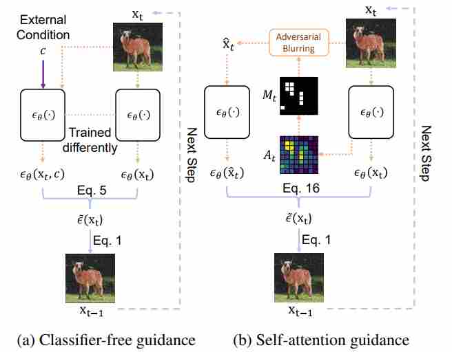
How to construct the bad branch.
- Run the model once to obtain self-attention maps \(A_t\) (or a derived mask \(M_t\)).
Construct a perturbed latent \(\tilde{x}_t\) by blurring/noising the attended regions:
\[\begin{align} \tilde{x}_t \; & =\; \operatorname{Blur}(x_t\;,M_t) \\[10pt] \quad\text{or}\quad \tilde{x}_t \; & =\; (1-M_t)\odot x_t + M_t\odot \operatorname{Blur}(x_t). \end{align}\]- Run the model again (same $c$) to get the “bad” prediction \(u_\theta(\tilde{x}_t,t,c)\).
Guidance form. In the generic template:
\[u_{\text{SAG}} = u_\theta^{+} + \omega_{\text{sag}}(u_\theta^{+}-u_\theta^{-}).\]where
\[u_\theta^{+}=u_\theta(x_t,t,c),\qquad u_\theta^{-}=u_\theta(\tilde{x}_t,t,c),\]This matches our existing summary
\[g_{\text{SAG}}\approx u_\theta(x_t,t,c)-u_\theta(\tilde{x}_t,t,c)\]5.2.3 Perturbed Attention Guidance (PAG)
Idea. PAG constructs the “bad branch” by perturbing self-attention computation paths directly, instead of corrupting the latent in pixel/latent space. Concretely, it generates degraded-structure intermediates by substituting selected self-attention maps with an identity matrix, then guides sampling away from those degraded predictions.
PAG is explicitly motivated by the fact that CG/CFG “are often not applicable in unconditional generation or downstream tasks such as image restoration,” and targets improvements in both conditional and unconditional settings without extra modules/training.
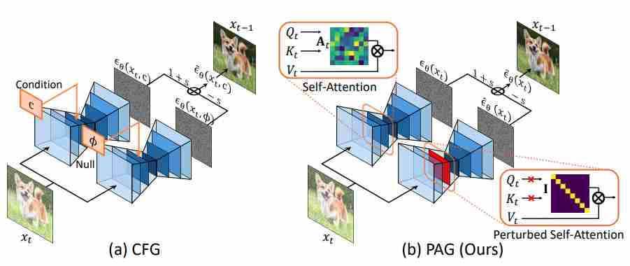
How to construct the bad branch.
Let a self-attention layer produce attention weights
\[W \;=\; \operatorname{softmax}!\Big(\frac{QK^\top}{\sqrt{d}}\Big)\in\mathbb{R}^{N\times N}.\]PAG defines a perturbed attention \(\widetilde{W}\), or applied only to a subset of layers/heads/tokens. Running the U-Net with \(\widetilde{W}\) removes token-to-token mixing and yields a structurally degraded prediction \(u_\theta^{-}\).
Guidance form.
\[u_{\text{PAG}} = u_\theta^{+} + \omega_{\text{pag}}(u_\theta^{+}-u_\theta^{-}).\]where
\[u_\theta^{+}=u_\theta(x_t,t,c;,W),\qquad u_\theta^{-}=u_\theta(x_t,t,c;,\widetilde{W}),\]5.2.4 Smoothed Energy Guidance (SEG)
Idea. SEG makes the “bad/unconditional-like” branch by smoothing the attention energy landscape, specifically by reducing the curvature of the attention energy. It is described as a “training- and condition-free approach” that (i) defines an energy for self-attention, (ii) reduces its curvature, and (iii) uses the resulting output as an unconditional prediction.
How to construct the bad branch (high-level).
- Define an attention-energy view of the self-attention mechanism.
- Apply Gaussian smoothing (controlled by a kernel parameter) to reduce curvature while keeping guidance scale fixed.
- Implement the smoothing efficiently via query blurring, which is stated to be equivalent to blurring the full attention weights but without quadratic token complexity.
Guidance form. SEG naturally fits the internal-contrast template by treating the smoothed-attention output as \(u^{-}\):
\[u_\theta^{+}=u_\theta(x_t,t,c;,\text{original attention}),\qquad u_\theta^{-}=u_\theta(x_t,t,c;,\text{smoothed attention}),\]and the total direction:
\[u_{\text{SEG}} = u_\theta^{+} + \omega_{\text{seg}}(u_\theta^{+}-u_\theta^{-}).\]Interpretationally: SAG/PAG degrade by removing information (blur or identity attention), while SEG degrades by flattening the attention energy landscape—reducing sharp, high-curvature “overconfident” attention peaks that often correlate with side effects at high guidance.
5.2.5 AutoGuidance
Idea. AutoGuidance replaces the unconditional baseline by a bad version of the model itself (smaller and/or under-trained), using the same conditioning, thereby avoiding the “task discrepancy” between conditional and unconditional branches. The paper explicitly states that it guides using “a smaller, less-trained version of the model itself rather than an unconditional model,” and that it “does not suffer from the task discrepancy problem because we use an inferior version of the main model itself as the guiding model, with unchanged conditioning.”
How to construct the bad branch. Train or obtain an inferior model \(u_\phi\) that solves the same conditional task but is deliberately weaker (capacity/time degradations). Then:
\[u_\theta^{+}(x_t,t,c)=u_\theta(x_t,t,c), \qquad u_\theta^{-}(x_t,t,c)=u_\phi(x_t,t,c).\]Guidance form (CFG with “bad model” instead of “uncond”).
\[u_{\text{AG}}(x_t,t,c) \;=\; u_\theta(x_t,t,c) \;+\; \omega_{\text{ag}}\Big(u_\theta(x_t,t,c)-u_\phi(x_t,t,c)\Big).\]The key intuition given in the paper: when the strong and weak models agree, the correction is small; when they disagree, the difference indicates a direction toward better samples.
5.3 Dynamic Guidance Scheduling and Calibration
Standard CFG uses a single global guidance weight throughout the entire reverse-time trajectory:
\[s_{\mathrm{cfg}}(x_t,t,y)=s_u(x_t,t)+w\big(s_c(x_t,t,y)-s_u(x_t,t)\big),\qquad w \ge 1.\]This “fixed-$w$” design is simple, but it implicitly assumes that:
1) the conditional–unconditional discrepancy is equally informative at all $t$, and
2) the magnitude of the guidance increment is naturally calibrated across timesteps and prompts.
Both assumptions are empirically false and conceptually misaligned with diffusion/flow sampling dynamics 7 8 9.
In the early high-noise stage, the state is dominated by noise:
\[x_t=\alpha_t x_0+\sigma_t\varepsilon,\qquad \mathrm{SNR}(t)=\frac{\alpha_t^2}{\sigma_t^2}\ll 1.\]and the conditional–unconditional score difference is
\[s_c-s_u=\nabla_{x_t}\log p_t(y\mid x_t).\]which does not provide fine mode-specific semantics; instead, it approximately reduces to a coarse global drift
\[s_c-s_u \approx \frac{\alpha_t}{\sigma_t^2}(\bar\mu_y-\mu),\]where \(\bar\mu_y\) is the class-weighted conditional mean and \(\mu\) is the unconditional mean. Therefore, large guidance at this stage mainly amplifies a global bias term rather than useful fine-grained semantic structure. As a result, CFG induces early direction shift and norm inflation, steering trajectories toward the scaled mean \(\omega\bar\mu_y\). If the conditional distribution contains a dominant mode, this early displacement reduces later occupancy of weaker attraction basins, so diversity is already compromised before genuine mode separation becomes active.
In the intermediate denoising regime, the conditional posterior over semantic modes becomes most sensitive to the current state $x_t$. In a two-mode mixture, if \(r_1(x_t)\) denotes the posterior responsibility of mode 1 along the discriminative direction \(u=\langle x_t,\mu_1-\mu_2\rangle\), then
\[\frac{\partial r_1}{\partial u}=a_t,r_1(1-r_1),\]where \(a_t\) increases as noise decreases, while \(r_1(1-r_1)\) is maximal before mode assignment saturates. Hence the intermediate stage is exactly where the conditional correction becomes most informative and mode-selective. Amplifying it with a larger guidance scale therefore helps trajectories commit more decisively to the appropriate attraction basin, rather than merely inducing a global bias as in the early stage.
In the high-SNR tail regime, posterior mode responsibilities are already saturated, so guidance no longer meaningfully contributes to mode selection. Locally inside a selected basin $k$, the conditional score reduces to a linear restoring field
\[s_c(x_t,t,y)\approx -\frac{x_t-\alpha_t\mu_k}{\alpha_t^2\sigma_y^2+\sigma_t^2},\]i.e., a force pulling the trajectory toward the local mode center. Since this local conditional field is sharper than the unconditional one, increasing the guidance scale mainly strengthens the contraction rate
\[\kappa_{\mathrm{cfg}}(t)=\lambda_c(t)+(w-1)\big(\lambda_c(t)-\lambda_u(t)\big),\]which accelerates the collapse of nearby trajectories within the same mode. Thus, large late-stage guidance contributes little new semantic information but increasingly suppresses fine-grained variability, making a low guidance scale the principled choice in the tail stage.
5.3.1 Adaptive Guidance (AG)
An key insight in AG 10 is that as the number of sampling steps increases, the similarity between the outputs of the unconditional branch and the conditional branch becomes progressively higher.
Adaptive Guidance (AG) 10 leverages this observation by dynamically deciding when to apply CFG and when to rely solely on the conditional branch. Let
\[\gamma_t = \frac{\epsilon_\theta(x_t, t, c) \cdot \epsilon_\theta(x_t,t, \varnothing)}{\|\epsilon_\theta(x_t, t, c)\|\cdot \|\epsilon_\theta(x_t,t, \varnothing)\|}\]denote the cosine similarity between conditional and unconditional network outputs. Empirically, $\gamma_t$ increases monotonically over time and approaches 1 toward the end of the process, indicating nearly perfect alignment.
AG introduces a threshold $\bar{\gamma}\in[0,1]$ to determine the switch point:
When $\gamma_t < \bar{\gamma}$, CFG is executed as usual—combining conditional and unconditional predictions to strongly enforce textual conditioning.
\[{\mathrm g}_{\text{total}} = {\mathrm g}_{\text{uncond}} + w\cdot ({\mathrm g}_{\text{cond}} - {\mathrm g}_{\text{uncond}})\]When $\gamma_t \ge \bar{\gamma}$, the model stops computing the unconditional branch, using only the conditional output for subsequent steps.
\[{\mathrm g}_{\text{total}} = {\mathrm g}_{\text{cond}}\]
This adaptive truncation maintains the semantic fidelity established during early denoising while removing redundant computations in the later phase.
5.3.2 β-CFG:
A fixed guidance scale $w$ across all denoising steps is inappropriate. β-CFG 11 introduces a time-dependent and normalized guidance mechanism to stabilize this process. It replaces the constant $w$ with a dynamic function $ \beta(t) $ and introduces a normalization exponent $ \gamma $ to control the magnitude of the conditional correction:
\[{\mathrm g}_{\text{total}} = {\mathrm g}_{\text{uncond}} + \beta(t)\,\frac{w\cdot ({\mathrm g}_{\text{cond}} - {\mathrm g}_{\text{uncond}})}{\|{\mathrm g}_{\text{cond}} - {\mathrm g}_{\text{uncond}}\|^\gamma}\]This modification simultaneously ensures the manifold structure at both ends of the diffusion path and gradient stability.
Beta-Distribution Scheduling. The first key component is the β-function weighting:
\[\beta(t) = \frac{t^{a-1}(1-t)^{b-1}}{B(a,b)}, \quad a,b>1.\]This curve is zero at both ends $(\beta(0)=\beta(1)=0)$ and peaks in the middle, forming a “weak–strong–weak” pattern. Such a schedule satisfies the boundary conditions required to keep trajectories on the data manifold:
Hence, early and late denoising steps use almost pure unconditional predictions (stabilizing start and end), while the mid-range receives strong conditional influence—the region most responsible for semantic formation. This design directly addresses the three-phase mechanism of diffusion sampling:
$\gamma$-Normalization: Gradient Rescaling Perspective
The second component, $\gamma$-normalization, controls the effective step size of the guidance. As we had discussed before, CFG can be viewed as performing gradient ascent on an implicit energy function
\[\mathcal{F}_{\text{CFG}} = \tfrac{1}{2}\|{\mathrm g}_{\text{cond}} - {\mathrm g}_{\text{uncond}}\|^2, \quad \nabla_{ {\mathrm g}_{\text{cond}} }\mathcal{F}_{\text{CFG}} = ({\mathrm g}_{\text{cond}} - {\mathrm g}_{\text{uncond}}).\]where the difference \(\Delta=\nabla_{ {\mathrm g}_{\text{cond}} }\mathcal{F}_{\text{CFG}}\) represents the gradient ascent direction. Multiplying by \(1/\|\Delta\|^\gamma\) therefore acts as a rescaling schedule: Large $|\Delta|$: down-scale the update to prevent gradient explosion, while Small $|\Delta|$ amplify subtle conditional cues to avoid vanishing.
This normalization stabilizes the dynamics of CFG, keeping the trajectory within a numerically safe and geometrically valid region.
5.3.3 CFG-Zero★ (Flow Matching): projection-based rescale + early-step zero-init
CFG-Zero★ targets flow-matching / rectified-flow style samplers, where CFG is applied to a predicted velocity field (or an equivalent direction). The central idea is that the unconditional branch can be recalibrated to better match the conditional prediction via a 1D projection, producing a more stable mixture.
Optimized scale via projection. Consider scaling the unconditional prediction by a scalar $s_t$:
\[\tilde{u}_u \triangleq s_t\, u_\theta(x_t,t,\varnothing).\]Choose $s_t$ by minimizing the squared mismatch between conditional and scaled-unconditional predictions:
\[s_t^\star = \arg\min_{s}\; \big\|u_\theta(x_t,t,c) - s\,u_\theta(x_t,t,\varnothing)\big\|_2^2.\]This is a one-variable least-squares problem. Expanding and differentiating:
\[\begin{aligned} f(s) &= \|u_c - s u_u\|_2^2 = \langle u_c - s u_u,\; u_c - s u_u\rangle,\\[10pt] \Longrightarrow\quad \frac{d f}{ds} &= -2\langle u_u,\;u_c - s u_u\rangle = -2\langle u_u,u_c\rangle + 2s\|u_u\|^2. \end{aligned}\]Setting $df/ds=0$ gives the closed form:
\[s_t^\star= \frac{\langle u_\theta(x_t,t,c),\;u_\theta(x_t,t,\varnothing)\rangle} {\|u_\theta(x_t,t,\varnothing)\|_2^2}.\]CFG is then applied between $u_c$ and the scaled unconditional $\tilde{u}_u$:
\[u_{\text{CFG-Zero★}} = \tilde{u}_u + \omega\Big(u_c-\tilde{u}_u\Big) = s_t^\star u_u + \omega\Big(u_c - s_t^\star u_u\Big).\]When $s_t^\star\approx 1$, it reduces to standard CFG. When $s_t^\star$ differs from 1, the method effectively performs a “projection-calibrated” mixture.
Zero-init at the earliest steps. Empirically, the first reverse steps can be particularly sensitive in flow-matching samplers. CFG-Zero★ therefore also advocates an early-step suppression (a “zero-init”) so that the dynamics do not overreact to poorly calibrated directions at the very beginning. In the unifying lens of (Dyn-CFG), this is again a stage-aware schedule:
\[\text{very-early steps: }\;\omega(t)\approx 0 \quad\Longrightarrow\quad u_{\text{dyn}}\approx \tilde{u}_u \;\text{(or even }0\text{)}.\]
6. Guidance via Measurements (Inverse Problems)
This chapter covers measurement-conditioned generation, where the “condition” is not semantic text/class labels, but observations produced by a known forward process (blur kernel, downsampling, masking, tomography operator, Fourier magnitude, etc.). Since we will discuss inverse problems in depth elsewhere, we only establish the unifying lens and the canonical inference-time templates used by diffusion/flow samplers. For more details, please check the following paper:
6.1 Problem Setup: Forward Model and Posterior
Let the unknown clean signal/image be \(x\in\mathbb{R}^d\). Measurements \(y\) are generated by a (typically known) operator:
\[y = A(x) + \eta, \qquad \eta \sim \mathcal{N}(0,\sigma_y^2 I),\]where \(A(\cdot)\) can be linear (matrix \(A\)) or nonlinear (e.g., phase retrieval magnitude). The inverse problem is to sample from (or approximate) the posterior
\[p(x \mid y) \;\propto\; p(x)\,p(y\mid x),\]where \(p(x)\) is the learned data prior (captured implicitly by the pretrained diffusion/flow model), and \(p(y\mid x)\) is the measurement likelihood induced by \(A\).
6.2 From “Energy Guidance” to Measurement Guidance
A key reason measurement guidance naturally appears as an additive correction is the log-posterior decomposition:
\[\nabla_x \log p(x\mid y) = \nabla_x \log p(x) + \nabla_x \log p(y\mid x).\]Equivalently, define a measurement energy
\[E_{\text{meas}}(x;y) \;=\; -\log p(y\mid x) \quad(\text{up to a constant}),\]then
\[\nabla_x \log p(x\mid y) = \nabla_x \log p(x) - \nabla_x E_{\text{meas}}(x;y).\]In diffusion / flow sampling, we do not operate directly on clean \(x_0\), but on noisy states \(x_t\). A practical and widely used template is to impose measurement consistency through a proxy clean estimate \(\widehat{x}(x_t,t)\) (often \(\hat{x}_0(x_t,t)\)):
\[\begin{align} & E_{\text{meas}}(x_t,t;y) \;\propto\; \big\|A\,\widehat{x}(x_t,t) - y\big\|_2^2 \\[10pt] \quad\Rightarrow\quad & u_{\text{ctrl}}(x_t,t) \;=\; u_{\text{base}}(x_t,t)\;-\;\lambda(t)\,\nabla_{x_t}E_{\text{meas}}(x_t,t;y). \end{align}\]Interpretation. Compared to CFG (which injects a semantic increment), measurement guidance injects a data-consistency increment. Both are instances of “base dynamics + guided correction,” but the guidance signal here is determined by physics / measurement operators rather than learned \(p(c\mid x)\).
6.3 Practical Forms of the Measurement Gradient
For Gaussian noise and linear \(A\), a common choice is
\[E_{\text{meas}}(x_t,t;y) = \frac{1}{2\sigma_y^2}\,\|A\,\widehat{x}(x_t,t) - y\|_2^2.\]Then, by chain rule,
\[\nabla_{x_t}E_{\text{meas}} = \frac{1}{\sigma_y^2}\,J_{\widehat{x}}(x_t,t)^\top\,A^\top\big(A\,\widehat{x}(x_t,t)-y\big),\]where \(J_{\widehat{x}}\) is the Jacobian of \(\widehat{x}\) wrt \(x_t\). In implementations one typically avoids explicit Jacobians and uses autodiff to backprop through \(\widehat{x}\) and $A$.
For nonlinear \(A(\cdot)\), replace \(A\,\widehat{x}\) by \(A(\widehat{x})\) and backprop through \(A(\cdot)\) if it is differentiable (or through a differentiable surrogate if not).
6.4 Two Canonical Templates: Soft vs Hard Data Consistency
Soft consistency: gradient correction (MAP / posterior-inspired). At each sampling step, do a base update, then take a small step that reduces measurement residual.
Hard consistency: projection / proximal enforcement. When the feasible set is easy to enforce,
\[\mathcal{S}=\{x:\;A x=y\}\quad\text{or}\quad \mathcal{S}=\{x:\;\|Ax-y\|\le \epsilon\},\]one can apply a projection/prox step after the base update:
\[x \leftarrow x + \Delta t\,u_{\text{base}}(x,t), \qquad x \leftarrow \Pi_{\mathcal{S}}(x).\]This is the operator-splitting view: prior step (diffusion/flow) + data-consistency step (projection/prox).
7. Inference-time Image Editing
This chapter focuses on inference-time editing: we keep the pretrained diffusion model fixed (no fine-tuning), and we do not run an outer-loop optimization over prompts/latents (so methods like Null-text optimization / prompt embedding optimization are not included). Instead, we edit by intervening directly in the sampling dynamics—either by choosing a special initialization, or by modifying intermediate tensors (attention/features), or by enforcing region constraints.
Throughout, let the diffusion model be written in the standard noise-prediction form:
\[q(x_t\mid x_0)=\mathcal N\!\left(\sqrt{\bar\alpha_t},x_0,\;(1-\bar\alpha_t)\mathbf I\right),\qquad \epsilon_\theta(x_t,t,c)\approx \epsilon\]and the usual estimate of the clean image from a noisy latent:
\[\hat x_0(x_t,t,c)=\frac{x_t-\sqrt{1-\bar\alpha_t}\,\epsilon_\theta(x_t,t,c)}{\sqrt{\bar\alpha_t}}.\]This identity (or its latent-space analogue in LDM/Stable Diffusion) is the “bridge” that lets editing losses (which usually live on clean images) act during denoising. You’ll see \(\hat x_0\) appear repeatedly, especially in CLIP-guided local editing.
We organize inference-time editing into four routes (matching your TOC):
- 7.1 Noise-perturb-then-denoise: edit by choosing how far you “forget” the source, then re-denoise under a new condition.
- 7.2 Attention routing control: edit by rewriting where the model attends (cross/self attention).
- 7.3 Feature and state injection: edit by injecting intermediate states/features from a reference trajectory.
- 7.4 Mask region control: edit by explicitly constraining “keep background / only change ROI”.
7.1 Noise-perturb-then-denoise
The simplest (and still surprisingly powerful) inference-time editing idea is:
- Start from a real/source image \(x^{src}\).
- Corrupt it to some noise level \(t_0\) (or \(\sigma\) in continuous SDE notation).
- Run the reverse process under a new condition \(c^{tgt}\) (new prompt, new guidance, etc.).
Intuitively, \(t_0\) controls the realism–faithfulness trade-off:
- small noise: preserve identity/structure strongly, but limited semantic change;
- large noise: allow bigger edits, but risk losing the source structure.
This is exactly the principle articulated by SDEdit 12: “add noise, then denoise with the generative prior” to balance faithfulness and realism without task-specific training.
Core idea. SDEdit (Stochastic Differential Editing) uses a diffusion/SDE generative prior to “project” a user-provided input (stroke image, composited image, corrupted edit, etc.) back onto the natural-image manifold: add enough noise to wash out artifacts but keep coarse structure, then denoise.
Discrete-time (DDPM-style) view. Pick a timestep \(t_0\). Noise the input:
\[x_{t_0}=\sqrt{\bar\alpha_{t_0}}\,x^{src}+\sqrt{1-\bar\alpha_{t_0}}\,\epsilon,\quad \epsilon\sim\mathcal N(0,I).\]Then run reverse sampling from \(t=t_0\to 0\) with the model (optionally conditioned on text or other signals):
\[x_{t-1}\sim p_\theta(x_{t-1}\mid x_t,\;c^{tgt}).\]Continuous-time (SDE) intuition. In SDEdit’s original framing, you perturb the input by forward SDE to time \(\sigma\), then simulate the reverse SDE back to \(\sigma=0\), thereby increasing likelihood under the score-based prior.
7.2 Attention Routing Control
In text-to-image diffusion (LDM/SD), the U-Net (or DiT-like backbone) contains attention layers that route information:
- Cross-attention ties spatial features to text tokens.
- Self-attention propagates spatial/global coherence inside the image latent.
A generic attention block (single head, for simplicity):
\[\mathrm{Attn}(Q,K,V)=\mathrm{softmax}\!\left(\frac{QK^\top}{\sqrt d}\right)V.\]Editing by “attention control” means: during sampling, we replace or mix some of \((Q,K,V)\) or the attention weights, so that the target trajectory inherits desired layout/structure from a source trajectory. Prompt-to-Prompt is the canonical cross-attention example.
7.2.1 Cross-Attention Map Injection (Prompt-to-Prompt)
Problem Prompt-to-Prompt 13 addresses. In large text-conditioned diffusion models, small prompt edits often yield totally different images. P2P aims to edit semantics while preserving layout/structure, using text only (no manual mask required).
Key observation. Cross-attention maps are strongly correlated with where each word appears in the image; thus, controlling cross-attention lets you control layout/token grounding.
Mechanism (high-level, but faithful).
Run diffusion with the source prompt \(c^{src}\), and record cross-attention maps \({A^{src}_{t,\ell}}\) (for timesteps \(t\), layers \(\ell\)).
Run diffusion with the edited prompt \(c^{tgt}\), but inject/replace some cross-attention maps (or parts corresponding to preserved tokens) with those from the source run, producing \({A^{edit}_{t,\ell}}\). A convenient way to write the intervention is a masked merge:
\[A^{edit}_{t,\ell} = M \odot A^{src}_{t,\ell} + (1-M)\odot A^{tgt}_{t,\ell},\]Continue denoising; the target sample is now “pulled” to keep the original layout for preserved words while allowing changes for edited words.
where $M$ selects tokens (or token-to-pixel rows/columns) you want to preserve. (P2P implements several variants of this idea—replacement/refinement/reweighting—depending on edit type.)
| Operation Type | Example (Source → Target) | Attention Map Modification |
|---|---|---|
| Token Replacement | “a dog on the grass” → “a cat on the grass” | $\tilde{A}_{:,col(dog)} = A_t[:,col(cat)]$ Other columns unchanged, copy from $A_s$ |
| Modifier Insertion | “a dog” → “a brown dog” | $\tilde{A} = [A_s[:,a], A_t[:,brown], A_s[:,dog]]$ Re-normalize after insertion |
| Degree Word Insertion | “a cute dog” → “a very cute dog” | $\tilde{A}_{:,cute}=(1+\lambda)A_s[:,cute]$ $\tilde{A}_{:,very}=\eta A_s[:,cute]$ |
| Token Deletion | “a brown dog” → “a dog” | Delete “brown” column: $\tilde{A}=[A_s[:,a],A_s[:,dog]]$ |
| Attribute Strengthening | “a cute dog” → “a very cute dog” or enhance “cute” effect | $\tilde{A}_{:,cute}=(1+\lambda)A_s[:,cute]$ |
| Attribute Weakening | “a very cute dog” → “a cute dog” | $\tilde{A}_{:,cute}=(1-\lambda)A_s[:,cute]$ |
| Token Reordering | “a red big dog” → “a big red dog” | Reorder columns: $\tilde{A}=[A_s[:,a],A_s[:,big],A_s[:,red],A_s[:,dog]]$ |
| Style Injection | “a dog” → “a dog in watercolor style” | High-level blending: $\tilde{A}^{(l)}=(1-\alpha)A_s^{(l)}+\alpha A_t^{(l)}$ ($\alpha≈0.2$) |
Interpretation. For a spatial position (i), the cross-attention output is \(y_i=\sum_j a_{ij}v_j\). Replacing \(a_{ij}\) for specific tokens \(j\) preserves the spatial “where” each word acts, while allowing the values \(v_j\) (from the new prompt) to change the “what”.
7.2.2 MasaCtrl: Mutual Self-Attention
The fundamental innovation of MasaCtrl is the transformation of the standard Self-Attention mechanism into Mutual Self-Attention.
Standard Self-Attention (in Stable Diffusion): Usually, a generated image queries its own features to refine texture and consistency.
\[\text{Attention}(Q, K, V) = \text{Softmax}\left(\frac{QK^T}{\sqrt{d}}\right)V\]Here, $Q, K, V$ all come from the same image being generated.
The Insight: To edit an image (e.g., changing a dog’s pose from sitting to standing) without losing identity, we need two things: Structure/Layout: Defined by the new text prompt (Target), and Appearance/Texture: Defined by the original image (Source).
Mutual Self-Attention Mechanism: MasaCtrl decouples these roles. It uses the Queries ($Q$) from the target image (to determine where things are and what shape they take) and the Keys ($K$) and Values ($V$) from the source image (to determine what they look like).
\[\text{Attention}(Q_{tgt}, K_{src}, V_{src})\]
The workflow involves running two diffusion processes in parallel (or sequentially): a Source Branch and a Target Branch.
Step 1: Source Image Processing (Reference). The model performs DDIM inversion (for real images) or generation (for synthetic images) using the original prompt ($P_{src}$).
During this process, the algorithm caches (saves) the $K_{src}$ and $V_{src}$ matrices from specific Self-Attention layers in the U-Net.
These matrices represent the “texture bank” of the original subject and background.
Step 2: Target Image Layout Generation (Early Steps). The model starts denoising the target image using the edited prompt ($P_{tgt}$, e.g., “a running corgi”).
Crucial Strategy: For the initial denoising steps (from $T$ down to a threshold $S$), the model uses Standard Self-Attention.
The broad layout and pose (the non-rigid structure) are determined in the early stages of diffusion. By using the new prompt without interference, the model naturally generates the new shape (e.g., the “running” pose).
Step 3: Appearance Injection via MasaCtrl (Later Steps). Once the denoising process passes the threshold step $S$, the algorithm switches to Mutual Self-Attention.
In the decoder layers of the U-Net, the current spatial features of the target image are projected into Queries ($Q_{tgt}$). Instead of looking at itself, the model queries the cached $K_{src}$ and $V_{src}$.
Result: The pixels in the “running dog” shape ($Q_{tgt}$) “look up” the texture of the “sitting dog” ($K_{src}, V_{src}$) and paint the original fur pattern onto the new body.
To ensure high-quality results, MasaCtrl employs two specific strategies, MasaCtrl is not applied at every step.
- Early steps: Vanilla attention (to form new structure).
- Late steps: Mutual attention (to copy original texture).
It is largely applied in the Decoder layers of the U-Net, which contain high-resolution semantic details, rather than the Encoder layers which handle abstract composition.
7.2.3 KV Caching and Reuse (Background/Structure Preservation)
A more structural form of attention intervention is to cache and reuse key/value tensors (or subsets of them) to preserve parts of the scene. A recent example is KV-Edit, which targets transformer-based diffusion (DiT-like) attention: it caches background key-value pairs so that editing focuses on the foreground while the background is reconstructed from reused memory.
At a high level, the intervention looks like:
\[\begin{align} & (K,V) \leftarrow \big(K^{\text{reuse}},V^{\text{reuse}}\big)\ \ \text{for background tokens}, \\[10pt] & (K,V) \leftarrow (K^{\text{new}},V^{\text{new}})\ \ \text{for editable tokens}. \end{align}\]This creates a decoupling inside attention: the “preserve set” is forced to follow a previously cached representation, while the “edit set” remains free to adapt to the new prompt/constraint.
When this is preferable to P2P. Attention-map injection (P2P) is most natural for token-level semantic edits. KV reuse can be more direct when the objective is perfect background preservation or structure locking.
7.2.4 Unified Attention Control (infEdit)
infEdit targets a very practical pain point: many attention-based editors rely on inversion steps; infEdit proposes inversion-free editing while still preserving structure, by unifying cross- and self-attention control into a single mechanism called Unified Attention Control (UAC).
How UAC is formulated (as written in the paper). They explicitly decompose attention into two operations:
Attention Modulation: replace the softmax attention weights \(P=\mathrm{softmax}(QK^\top/\sqrt{d})\) with an interpolated weight map:
\[P_{\mathrm{mod}}=\eta P + (1-\eta)P',\]where $P’$ is an “alternative” attention distribution (e.g., from the reference/source context), and \(\eta\in[0,1]\) controls how much to preserve.
Attention Merging: after attention produces outputs, merge reference and target attention outputs:
\[A_{\mathrm{merge}}=\gamma\cdot(PV) + (1-\gamma)\cdot(P'V'),\]with \(\gamma\in[0,1]\).
These two knobs—$\eta$ and $\gamma$—let infEdit unify “preserve vs edit” behaviors across attention types (cross/self) in one framework.
Why this matters conceptually. P2P is primarily cross-attention injection; MasaCtrl emphasizes self-attention consistency. UAC provides a single algebraic language to do both, and then schedule \((\eta,\gamma)\) across layers/timesteps to balance preservation and edit strength.
Where infEdit is useful.
- When you want strong structure preservation but prefer to avoid explicit inversion pipelines.
- When both token grounding and internal spatial coherence must be controlled jointly.
7.3 Feature / State Injection
Attention control edits “routing weights”. Feature/state injection goes deeper: it directly injects intermediate U-Net features or attention tensors from a reference run into the edited run.
You can view it as: run a reference trajectory \({x_t^{ref}}\) (often induced by an input image), and a target trajectory \({x_t^{tgt}}\). At certain points in the network graph, replace:
\[h^{tgt}_{t,\ell}\leftarrow \mathcal I\big(h^{tgt}_{t,\ell}\,,h^{ref}_{t,\ell}\big),\]where \(\mathcal I\) is an injection operator (copy, blend, masked blend, etc.).
7.3.1 Plug-and-Play Diffusion Features (PnP)
The core of Plug-and-Play (PnP) Diffusion Features can be summarized as a tuning-free, zero-shot framework that achieves high-fidelity image editing by manipulating the internal representations of a pre-trained Diffusion Model.
The algorithm is based on the discovery that intermediate features in the Diffusion UNet (specifically during the decoding stage) carry critical information:
- Spatial Features: Represent fine-grained texture, shape, and precise spatial layout.
- Self-Attention Maps: Capture the semantic layout and the structural relationship between different parts of the image.
PnP operates through a three-step process without any model training or optimization:
- Step 1: DDIM Inversion: The source image is inverted into the latent noise space ($z_T$) to ensure the generation process starts from a point that can reconstruct the original image.
- Step 2: Source Branch (Extraction): The model performs a standard denoising pass using the source prompt. During this pass, it “records” and saves the Spatial Features ($f$) and Self-Attention Maps ($A$) from the UNet at each timestep $t$.
Step 3: Target Branch (Injection): A second denoising pass is performed using the Target Prompt. In this branch, the algorithm overwrites its own features with the saved features from the source branch:
\[\begin{align} & f_{target} \leftarrow f_{source} \quad \text{Spatial Feature Injection} \\[10pt] & A_{target} \leftarrow A_{source} \quad \text{Self-Attention Injection} \end{align}\]
The “Plug-and-Play” nature comes from the strategic application of injection:
- Layer-wise Control: Injection is typically applied only to the UNet Decoder layers, allowing the Encoder to remain flexible enough to interpret new text guidance.
- Time-wise Control: Features are injected only during the early-to-mid stages of the denoising process (where structure is formed) and stopped in the final steps to allow the model to produce clean, artifact-free pixels.
In essence, PnP treats the internal features of a diffusion model as a “structural anchor,” forcing the new generation to grow within the bones of the original image.
7.3.2 FreeControl
Part III — Inference-time Optimization
Inference-time Optimization, also known as Optimization-Based Inference-Time Control, this category also operates at inference time, but unlike the previous one (Part II), it introduces additional optimization or iterative correction during sampling, while still leaving model parameters unchanged. The optimization target may involve rewards, constraints, energies, reconstruction objectives, or external differentiable guidance. This category is especially relevant for reward-guided, energy-guided, or test-time optimization methods.
8. Optimizing Inversion Variables: Reconstructing a Given Image
Prompt-to-Prompt (P2P) enables semantic-level image editing by manipulating token-specific cross-attention maps between a source prompt $c_{\text{src}}$ and a target prompt $c_{\text{tgt}}$. When the image is originally generated by the diffusion model, P2P can reuse the same initial noise latent $x_T$ and then control how attention maps are replaced, refined, or reweighted during the denoising process. In this setting, the unchanged parts of the prompt can preserve their spatial correspondences, while edited tokens modify only the desired semantic regions.
However, this assumption breaks down for real-image editing. For a real image $I$, we are given the final clean image, but we do not know the latent noise $x_T$ that would reconstruct it under the pretrained diffusion sampler. Therefore, before attention-based editing methods such as P2P can be applied to real images, one must first solve an inversion problem:
Given a real image $I$ and its source prompt $c_{\text{src}}$, find a latent trajectory $\{x_t\}_{t=0}^{T}$ such that the pretrained diffusion model can reconstruct $I$ and then edit it as if it were a model-generated image.
This problem is known as diffusion inversion. In latent diffusion models such as Stable Diffusion, the image is first mapped into the VAE latent space,
\[x_0 = \mathcal E(I),\]where $\mathcal E$ is the image encoder. The goal is then to find a noisy latent $x_T$ and, in more advanced methods, additional auxiliary variables, such that DDIM sampling from $x_T$ reconstructs $x_0$ with high fidelity.
This section focuses on inversion methods that do not retrain the diffusion model weights. Instead, they optimize or modify the variables used during inversion and sampling. The technical evolution is:
- DDIM Inversion: directly reverse the deterministic DDIM sampler to estimate $x_T$.
- Null-Text Inversion (NTI): keep the model and conditional prompt fixed, but optimize the unconditional CFG embedding at each timestep.
- Negative-Prompt Inversion (NPI): remove NTI’s per-step optimization by replacing the null-text embedding with the source-prompt embedding.
The central tension is reconstruction fidelity versus editing flexibility. A good inversion should not merely copy the image; it should reconstruct the source image while keeping the conditional prompt interface intact, so that subsequent prompt-based editing remains meaningful.
8.1 DDIM Inversion
DDIM Inversion is the most basic inversion method for deterministic diffusion sampling. DDIM constructs a non-Markovian generative process that can use the same trained denoising network as DDPM, while allowing deterministic sampling when the stochasticity parameter is set to $\eta=0$. This deterministic property makes it possible to approximately reverse the sampling trajectory.
Let $\bar\alpha_t$ denote the cumulative noise schedule:
\[\bar\alpha_t = \prod_{s=1}^{t} \alpha_s, \qquad \alpha_s = 1-\beta_s.\]Given a noisy latent $x_t$ and a noise prediction model $\epsilon_\theta(x_t,t,c)$ conditioned on prompt embedding $c$, the predicted clean latent is
\[\hat{x}_0^{(t)} = \frac{x_t-\sqrt{1-\bar\alpha_t}\,\epsilon_\theta(x_t,t,c)} {\sqrt{\bar\alpha_t}}.\]For deterministic DDIM sampling, one step from $t$ to $t-1$ is
\[x_{t-1} = \sqrt{\bar\alpha_{t-1}}\hat{x}_0^{(t)} + \sqrt{1-\bar\alpha_{t-1}}\epsilon_\theta(x_t,t,c).\]This equation defines the reverse denoising direction. DDIM Inversion applies the same relation in the opposite direction. Starting from the clean latent
\[x_0 = \mathcal E(I),\]we iteratively estimate increasingly noisy latents:
\[x_{t+1} \approx \sqrt{\bar\alpha_{t+1}}\hat{x}_0^{(t)} + \sqrt{1-\bar\alpha_{t+1}}\epsilon_\theta(x_t,t,c),\]where
\[\hat{x}_0^{(t)} = \frac{x_t-\sqrt{1-\bar\alpha_t}\epsilon_\theta(x_t,t,c)} {\sqrt{\bar\alpha_t}}.\]After iterating from $t=0$ to $T-1$, we obtain an estimated terminal latent $x_T^{\text{DDIM}}$. Sampling from this latent with the same prompt should approximately reconstruct the original image:
\[x_T^{\text{DDIM}} \;\xrightarrow{\text{DDIM sampling with }c}\; \hat{x}_0 \approx x_0.\]The key word is approximately. DDIM Inversion is not an exact inverse of the denoising process. Its accuracy depends on the assumption that the model’s predicted noise field changes smoothly between adjacent timesteps. Informally, one assumes that
\[\epsilon_\theta(x_t,t,c) \approx \epsilon_\theta(x_{t+1},t+1,c),\]so that the same predicted direction can be used to move both backward and forward along the trajectory. This approximation becomes imperfect when the timestep interval is large, the image is outside the model’s learned manifold, or classifier-free guidance strongly changes the denoising vector field.
For synthetic images generated by the same model, DDIM Inversion can often recover a usable latent code. For real images, however, several sources of error accumulate:
- Model mismatch: a real image may not lie exactly on the model’s generative manifold.
- Autoencoder distortion: in latent diffusion, $x_0=\mathcal E(I)$ is already an approximate latent representation of the image.
- Discretization error: practical samplers use a small number of inference steps, such as 50 or fewer, rather than the full training-time schedule.
- Guidance mismatch: high classifier-free guidance modifies the sampling dynamics and makes the inverse trajectory less stable.
As a result, DDIM Inversion is fast and simple, but its reconstruction quality is often insufficient for precise real-image editing. The reconstructed image may preserve the global layout but lose fine details, object identity, texture, or exact geometry. This limitation motivates optimization-based methods such as Null-Text Inversion.
8.2 Null-Text Inversion (NTI)
Null-Text Inversion (NTI) is an optimization-based method designed to improve real-image reconstruction while preserving the editability of prompt-based diffusion models. Its key idea is not to fine-tune the U-Net, the VAE, or the conditional prompt embedding. Instead, NTI optimizes only the unconditional embedding used in classifier-free guidance (CFG), also called the null-text embedding .
This design is important. If one directly optimizes the conditional prompt embedding or the model weights, the reconstructed image may become highly faithful but less editable, because the prompt representation itself may overfit to the input image. NTI avoids this by keeping the meaningful source prompt fixed and moving only the unconditional branch.
Stage I: Pivotal DDIM Inversion. The first stage constructs a pivotal trajectory using DDIM Inversion. Given a real image $I$ and its source prompt $c_{\text{src}}$, we first encode the image into the latent space:
\[x_0^\star = \mathcal E(I).\]Then DDIM Inversion is applied with the source prompt to obtain a trajectory
\[{x_0^\star,x_1^\star,\ldots,x_T^\star}.\]This trajectory is called “pivotal” because it acts as an anchor path for later optimization. Instead of asking the sampler to directly reconstruct the image from an arbitrary latent, NTI asks each denoising step to remain close to the corresponding step on this reference trajectory.
The terminal latent $x_T^\star$ provides the starting noise for reconstruction and editing. The full sequence ${x_t^\star}$ provides step-wise supervision for the null-text optimization stage.
Stage II: Optimizing the Null-Text Embedding. In classifier-free guidance, the guided noise prediction is usually written as
\[\epsilon_{\text{CFG}}(x_t,t,c,\emptyset) = \epsilon_\theta(x_t,t,\emptyset) + w\left[ \epsilon_\theta(x_t,t,c) - \epsilon_\theta(x_t,t,\emptyset) \right],\]where:
- $c$ is the conditional prompt embedding;
- $\emptyset$ is the null-text, or unconditional, embedding;
- $w$ is the guidance scale.
For ordinary text-to-image generation, $\emptyset$ is simply the embedding of an empty prompt. NTI replaces this fixed empty-prompt embedding with a timestep-dependent optimized embedding:
\[\emptyset \quad\longrightarrow\quad \emptyset_t.\]The guided prediction becomes
\[\epsilon_{\text{NTI}}(x_t,t,c,\emptyset_t) = \epsilon_\theta(x_t,t,\emptyset_t) + w\left[ \epsilon_\theta(x_t,t,c) - \epsilon_\theta(x_t,t,\emptyset_t) \right].\]The DDIM sampling step using this guided prediction is
\[\operatorname{DDIMStep}(x_t,t,c,\emptyset_t) = \sqrt{\bar\alpha_{t-1}}\hat{x}_0^{(t)} + \sqrt{1-\bar\alpha_{t-1}}\epsilon_{\text{NTI}}(x_t,t,c,\emptyset_t),\]where
\[\hat{x}_0^{(t)} = \frac{x_t-\sqrt{1-\bar\alpha_t}\epsilon_{\text{NTI}}(x_t,t,c,\emptyset_t)} {\sqrt{\bar\alpha_t}}.\]The optimization objective is to make the denoising step from $x_t^\star$ match the corresponding previous latent on the pivotal trajectory:
\[\boxed{ \min_{\emptyset_t} \left\| \operatorname{DDIMStep}(x_t^\star,t,c_{\text{src}},\emptyset_t) - x_{t-1}^\star \right\|_2^2 }\]In practice, NTI optimizes a separate null-text embedding for each timestep:
\[\{\emptyset_T^\star,\emptyset_{T-1}^\star,\ldots,\emptyset_1^\star\}.\]The U-Net parameters remain frozen. The VAE remains frozen. The conditional prompt embedding $c_{\text{src}}$ remains frozen. Only the unconditional embeddings used inside CFG are optimized.
This is the central insight of NTI: The reconstruction error is corrected through the unconditional branch, while the conditional branch remains semantically meaningful for editing.
After optimization, reconstruction starts from $x_T^\star$ and uses the optimized null-text embeddings during DDIM sampling:
\[x_T^\star \xrightarrow{ \text{DDIM sampling with }(c_{\text{src}},\emptyset_t^\star,w) } \hat{x}_0 \approx x_0^\star.\]The reconstructed latent can then be decoded:
\[\hat I = \mathcal D(\hat{x}_0),\]where $\mathcal D$ is the VAE decoder.
The reason NTI works is that classifier-free guidance depends on the difference between the conditional and unconditional predictions:
\[\epsilon_\theta(x_t,t,c) - \epsilon_\theta(x_t,t,\emptyset_t).\]Changing $\emptyset_t$ changes the effective guidance direction without changing the source prompt itself. Thus, the null-text embedding acts as a per-timestep correction variable. It absorbs errors caused by DDIM inversion, numerical discretization, and imperfect model predictions.
Compared with direct latent optimization, NTI has a better editing interface. The source prompt still represents the semantic content of the image. Therefore, editing methods such as Prompt-to-Prompt can still replace or modify token-specific attention maps in a meaningful prompt space.
Compared with model fine-tuning, NTI is also lightweight. It does not modify the pretrained diffusion model and does not require a dataset. The cost is that NTI performs iterative optimization for each input image, which can be slow.
8.3 Negative-Prompt Inversion (NPI)
Negative-Prompt Inversion (NPI) is a training-free and optimization-free alternative to Null-Text Inversion. It observes that the optimized null-text embeddings found by NTI can often be approximated by the embedding of the source prompt itself. Based on this observation, NPI replaces the null-text embedding in CFG with the source-prompt embedding, thereby achieving much faster inversion while retaining reconstruction quality close to NTI in many cases.
The motivation is simple. NTI improves reconstruction by finding an optimized unconditional embedding $\emptyset_t^\star$ such that the guided denoising trajectory matches the DDIM inversion trajectory. NPI asks whether we can avoid this optimization. Its answer is:
\[\emptyset_t^\star \approx c_{\text{src}}.\]Thus, instead of optimizing $\emptyset_t$, NPI directly uses the source prompt embedding as the negative-prompt embedding.
Reconstruction with NPI. Recall the CFG prediction:
\[\epsilon_{\text{CFG}}(x_t,t,c,\emptyset) = \epsilon_\theta(x_t,t,\emptyset) + w\left[ \epsilon_\theta(x_t,t,c) - \epsilon_\theta(x_t,t,\emptyset) \right].\]For reconstructing the source image, NPI sets both the conditional prompt and the negative prompt to the source prompt:
\[c = c_{\text{src}}, \qquad \emptyset = c_{\text{src}}.\]Substituting this into CFG gives
\[\begin{aligned} \epsilon_{\text{NPI-rec}}(x_t,t,c_{\text{src}}) &= \epsilon_\theta(x_t,t,c_{\text{src}}) + w\left[ \epsilon_\theta(x_t,t,c_{\text{src}}) - \epsilon_\theta(x_t,t,c_{\text{src}}) \right] \\[10pt] &= \epsilon_\theta(x_t,t,c_{\text{src}}). \end{aligned}\]Therefore, during reconstruction, CFG collapses to the conditional prediction itself. The guidance scale no longer changes the prediction, because the conditional and negative branches are identical.
This is why NPI can reconstruct efficiently. It does not run a per-timestep optimization loop. It simply performs DDIM Inversion and DDIM sampling while replacing the null-text embedding with the source-prompt embedding. The NPI paper reports that this avoids backpropagation and can run at roughly the same speed as DDIM Inversion, while being much faster than NTI ([CVF开放存取][4]).
Editing with NPI. For editing, the conditional prompt is changed from the source prompt to the target prompt:
\[c_{\text{src}} \quad\longrightarrow\quad c_{\text{tgt}}.\]However, NPI does not use the empty prompt as the unconditional branch. Instead, it uses the source prompt as the negative prompt:
\[\emptyset = c_{\text{src}}.\]Thus, the guided prediction during editing becomes
\[\begin{aligned} \boxed{ \epsilon_{\text{NPI-edit}}(x_t,t,c_{\text{tgt}},c_{\text{src}}) = \epsilon_\theta(x_t,t,c_{\text{src}}) + w\left[ \epsilon_\theta(x_t,t,c_{\text{tgt}}) - \epsilon_\theta(x_t,t,c_{\text{src}}) \right]. } \end{aligned}\]This equation explains the name Negative-Prompt Inversion. The source prompt is placed in the negative-prompt branch of CFG. It serves as the reference direction to be subtracted from the target direction.
Equivalently, the update direction can be interpreted as:
\[d_{\text{edited}} = {d_{\rm source}} + w \cdot (d_{\rm target} - d_{\rm source}).\]When $w=1$, this reduces to the target-prompt prediction:
\[\epsilon_{\text{NPI-edit}} = \epsilon_\theta(x_t,t,c_{\text{tgt}}).\]When $w>1$, the sampler moves beyond the source prompt toward the target prompt. This is analogous to ordinary CFG, but instead of moving away from an empty prompt, NPI moves away from the source prompt.
This design is especially suitable for real-image editing. The source prompt anchors the original image content, while the target prompt introduces the desired semantic change. When combined with attention-control methods such as Prompt-to-Prompt, NPI can preserve the source image structure while enabling prompt-level editing.
NPI can be understood as a zero-optimization approximation to NTI. NTI learns timestep-wise embeddings:
\[\{\emptyset_t^\star\}_{t=1}^{T} = \arg \min_{ {\emptyset_t} } \sum_t \left\| \operatorname{DDIMStep}(x_t^\star,t,c_{\text{src}},\emptyset_t) - x_{t-1}^\star \right\|_2^2.\]NPI replaces these optimized embeddings with the source-prompt embedding:
\[\emptyset_t^\star \approx c_{\text{src}}.\]Thus, the methodological difference is:
\[\boxed{ \text{NTI: learn } \emptyset_t^\star \text{ by optimization;} \qquad \text{NPI: approximate } \emptyset_t^\star \text{ by } c_{\text{src}}. }\]This approximation greatly reduces computation because it removes iterative optimization and backpropagation. However, it also means NPI may be less precise than NTI when the source image contains details that are not well captured by the source prompt, or when the DDIM inversion trajectory has significant accumulated error.
Part IV — Post-Training For Concept Customization and Consistency Preservation
The previous parts focused on controlling a fixed generator at inference time—by modifying guidance directions, manipulating attention or features, solving inversion variables, or imposing external constraints during sampling. We now move to a different but equally important regime: post-training control. Here, the goal is not merely to steer a single sampling trajectory, but to extend a pretrained generative model so that it can recognize, preserve, and reuse a newly specified concept across many future generations.
This regime is especially central to personalization and identity-consistent generation. Given only a few reference images of a subject, object, style, or character, the model must acquire a reusable representation of that concept while still preserving the prior knowledge and editability of the base model. Different methods mainly differ in where this new concept is stored: a learned token embedding, the full model weights, a low-rank parameter delta, a cross-attention modification, or an external image-conditioned adapter. In this part, we first study methods that require concept-specific retraining, and then contrast them with training-free approaches that extract and inject concept information directly at inference time.
10. Retraining-Based Personalization for New Concept Injection
Retraining-based personalization teaches a pretrained diffusion model a new visual concept from only a few reference images. This concept can be a specific person, pet, object, product, or artistic style. The general framework can be summarized as:
\[\require{color} \definecolor{lightred}{rgb}{1, 0.9, 0.9} \fcolorbox{red}{lightred}{$ \text{Few reference images} + \text{identifier token} \rightarrow \text{optimize a concept carrier}$ }\]The identifier token, such as sks, serves as a textual handle:
a photo of sks dog
sks dog wearing sunglasses
sks dog in watercolor style
The class word, such as dog, provides the general semantic prior, while sks points to the specific instance. The key question is:
This storage location is the concept carrier. Different retraining-based methods mainly differ in their chosen concept carrier:
| Method family | Concept carrier | Capacity |
|---|---|---|
| Textual Inversion / NeTI | learned token embeddings | Low |
| DreamBooth | U-Net / model weights | High |
| DreamBooth + LoRA | low-rank parameter deltas | Medium-High |
| Custom Diffusion / Perfusion | cross-attention K/V subspace | Medium |
| Mix-of-Show / Break-A-Scene | separated concept slots or concept banks | Variable |
Most methods still use a diffusion denoising objective:
\[\mathcal{L}_{\text{inst}} = \mathbb{E}_{x,t,\epsilon} \left[ \left\| \epsilon - \epsilon_\theta(x_t,t,c_{\text{inst}}) \right\|_2^2 \right],\]where \(c_{\text{inst}}\) is a personalized prompt such as “a photo of sks dog”. Some methods also add a prior preservation loss:
\[\mathcal{L} = \mathcal{L}_{\text{inst}} + \lambda \mathcal{L}_{\text{prior}}.\]Therefore, the main difference between these algorithms is often not the loss itself, but which parameters are optimized.
A small carrier, such as a token embedding, is lightweight and easy to share but has limited fidelity. A large carrier, such as the full U-Net, can encode richer identity and appearance details but is more expensive and more prone to overfitting. LoRA, adapter, and attention-based methods sit between these two extremes.
Thus, this section organizes retraining-based personalization by concept carrier:
- Token-embedding carriers: Textual Inversion, NeTI, P+ / XTI.
- Model-weight carriers: DreamBooth, AttnDreamBooth, DisenBooth.
- Parameter-efficient deltas: DreamBooth + LoRA, HyperDreamBooth, Orthogonal Adaptation.
- Cross-attention carriers: Custom Diffusion, Perfusion.
- Multi-concept carriers: Mix-of-Show, Break-A-Scene.
This carrier-based view gives a clearer structure than listing methods chronologically. It shows the central trade-off of retraining-based personalization:
Takeaway: higher carrier capacity means better fidelity, but higher cost and greater overfitting risk.
10.1 Token-Embedding-Based Concept Carriers
This family compresses the new concept into the text embedding space. Representative methods include:
- Textual Inversion
- Neural Textual Inversion / NeTI
- P+ / XTI
The core idea is:
\[\boxed{ \text{Concept carrier} = \text{learned token embeddings} }\]Instead of modifying the diffusion model itself, these methods introduce one or several special tokens and optimize their embeddings using a few reference images. The U-Net, VAE, and most of the text encoder remain frozen.
This makes the learned concept lightweight, stable, and easy to store or share. However, because the carrier is small, its capacity is limited. It is often effective for styles or coarse concepts, but less reliable for high-fidelity identity preservation or complex subject details.
In short, token-embedding-based methods trade capacity and fidelity for efficiency, stability, and model preservation.
10.1.1 Textual Inversion
Textual Inversion is an early and influential embedding-based concept injection method. Unlike DreamBooth, it does not fine-tune the diffusion model itself. Instead, it learns a new token embedding that represents the target concept.
Given a few images of a new subject, Textual Inversion introduces a special token, such as S*, and trains its embedding so that prompts like:
a photo of S* dog
S* dog in the snow
a painting of S* dog
can recall the new concept.
Core Objective: Textual Inversion uses the standard diffusion denoising loss:
\[\mathcal{L}_{\text{TI}} = \mathbb{E}_{x,t,\epsilon} \left[ \left| \epsilon - \epsilon_\theta(x_t,t,c_{S^*}) \right|_2^2 \right],\]where \(c_{S^*}\) is the text condition containing the learned token S*.
The key difference is that the diffusion model is frozen. During optimization, only the embedding vector of S* is updated.
Trainable and Frozen Parameters:
| Module | Status |
|---|---|
New token embedding S* | Fine-tuned |
| U-Net | Frozen |
| Text encoder | Frozen except the new token embedding |
| VAE | Frozen |
| Tokenizer | Extended with the new token |
So the new concept is compressed into a small learnable vector in the text embedding space.
Concept Carrier:
The concept carrier of Textual Inversion is:
\[\boxed{\text{the learned token embedding } e_{S^*}}\]Unlike DreamBooth, the model weights are not changed. The learned token acts as both the trigger and the storage location of the concept.
Carrier Capacity: Textual Inversion has low carrier capacity, because the concept must be represented by one or a few token embeddings.
This makes it lightweight and easy to store, but also limits how much visual detail it can capture. It usually works better for styles, textures, and broad visual concepts than for highly detailed identities or complex objects.
Advantages: The main advantage is efficiency. Textual Inversion only trains a tiny number of parameters, so it is cheap to train, easy to save, and easy to share.
It also preserves the original model well, because the U-Net and text encoder remain frozen. This greatly reduces the risk of model drift.
Limitations: The main weakness is limited fidelity. A single embedding often cannot encode all fine-grained details of a specific subject.
It is also sensitive to prompt design and initialization. If the learned token is poorly initialized or the training images are too diverse, the embedding may fail to capture a stable concept.
Compared with DreamBooth, Textual Inversion has better storage efficiency and less overfitting risk, but weaker subject fidelity and identity preservation.
In summary, Textual Inversion is a lightweight token-embedding-based concept injection method. Its concept carrier is compact and easy to manage, but its limited capacity makes it less suitable for high-fidelity identity or subject preservation.
10.1.2 P+ / Extended Textual Inversion
P+ / Extended Textual Inversion, or XTI, can be viewed as a layer-wise extension of Textual Inversion. It keeps the same basic philosophy as TI: the diffusion model is frozen, and the new concept is injected by optimizing textual embeddings rather than model weights.
The key difference is that Textual Inversion learns one token embedding shared by all U-Net cross-attention layers, while P+ learns a set of layer-specific textual embeddings:
\[P^+ = \{p_1,p_2,\dots,p_n\},\]where each \(p_i\) is injected into the corresponding cross-attention layer of the denoising U-Net. In Stable Diffusion 1.4, this means learning 16 token embeddings for 16 cross-attention layers.
Core Objective: XTI still uses the standard diffusion denoising loss:
\[\mathcal{L}_{\text{XTI}} = \mathbb{E}_{x,t,\epsilon} \left[ \left\| \epsilon - \epsilon_\theta(x_t,t,P^+_{S^*}) \right\|_2^2 \right],\]where \(P^+_{S^*}\) denotes the layer-wise textual condition learned for the new concept. Unlike TI, the concept is no longer compressed into a single embedding. Instead, different embeddings can specialize for different U-Net layers.
Trainable and Frozen Parameters:
| Module | Status |
|---|---|
| Per-layer token embeddings | Fine-tuned |
| U-Net | Frozen |
| Text encoder | Frozen except the new token embeddings |
| VAE | Frozen |
| Tokenizer | Extended with multiple new tokens |
Concept Carrier: The concept carrier of XTI is:
\[\boxed{\text{a set of layer-wise learned token embeddings } \{e_1,e_2,\dots,e_n\}}\]This is the main improvement over Textual Inversion. TI uses one compact carrier, while XTI uses multiple carriers distributed across the U-Net conditioning hierarchy.
Carrier Capacity: XTI has higher carrier capacity than TI, because each U-Net layer receives its own optimized textual condition.
This is important because different U-Net layers control different visual attributes. Coarse inner layers tend to influence object structure and geometry, while fine outer layers affect color, texture, and appearance. Therefore, XTI can distribute concept information more naturally across layers.
Advantages: The main advantage of XTI is better subject fidelity without modifying the diffusion model.
Compared with TI, XTI can reconstruct the target concept more accurately, converge faster, and preserve editability better. The paper reports that XTI uses far fewer optimization steps than TI while achieving better subject and text similarity.
Another advantage is controllability. Since the concept is represented layer by layer, XTI enables shape-style mixing: one concept can provide the coarse geometry, while another concept provides the fine appearance.
Limitations: XTI is still an embedding-based method, so its reconstruction ability is weaker than full model fine-tuning methods such as DreamBooth.
It also requires modifying the conditioning mechanism of the U-Net, because different layers must receive different textual embeddings. Therefore, it is less plug-and-play than standard Textual Inversion.
In summary, P+ / XTI extends Textual Inversion from a single-token carrier to a layer-wise multi-token carrier. It keeps the model-preserving advantage of TI, but significantly improves carrier capacity, subject fidelity, convergence speed, and controllability.
10.1.3 Neural Textual Inversion (NeTI)
NeTI, short for Neural Textual Inversion, further extends the idea of Textual Inversion and XTI. It still freezes the diffusion model, but replaces the fixed learned token embedding with a small neural mapper.
The motivation is simple: a personalized concept should not only depend on the U-Net layer, but also on the denoising timestep. Early denoising steps usually control coarse structure, while later steps refine local appearance and details. Therefore, NeTI represents a concept in a space-time textual conditioning space.
Instead of learning one token as in TI:
\[e_{S^*},\]or one token per U-Net layer as in XTI:
\[{e_1,e_2,\dots,e_L},\]NeTI learns a neural mapper:
\[\mathcal{M}(t,\ell) \rightarrow e_{t,\ell},\]where \(t\) is the denoising timestep and \(\ell\) is the U-Net cross-attention layer.
Core Objective: NeTI still uses the standard diffusion denoising loss:
\[\mathcal{L}_{\text{NeTI}} = \mathbb{E}_{x,t,\epsilon,\ell} \left[ \left\| \epsilon - \epsilon_\theta \left( x_t,t,c_{S^*}(\mathcal{M}(t,\ell)) \right) \right\|_2^2 \right].\]The key difference is that the optimized object is no longer a token embedding itself, but the parameters of the neural mapper \(\mathcal{M}\).
Trainable and Frozen Parameters:
| Module | Status |
|---|---|
| Neural mapper \(\mathcal{M}\) | Fine-tuned |
| U-Net | Frozen |
| Text encoder | Frozen |
| VAE | Frozen |
| Tokenizer | Extended with the new token |
Concept Carrier: The concept carrier of NeTI is:
\[\boxed{\text{the learned neural mapper } \mathcal{M}(t,\ell)}\]This mapper implicitly generates the concept embedding for each timestep and each U-Net layer.
Carrier Capacity: NeTI has higher carrier capacity than both TI and XTI.
TI uses one embedding for all layers and timesteps. XTI uses different embeddings for different layers, but they are still shared across all timesteps. NeTI further expands the carrier into a time-layer representation:
\[\begin{aligned} & \text{TI}: e \\[10pt] & \text{XTI}: e_\ell \\[10pt] & \text{NeTI}: e_{t,\ell} \end{aligned}\]This gives NeTI more expressive power for capturing both global structure and fine-grained details.
Additional Design: NeTI introduces a textual bypass. The mapper can output an additional residual vector that is added after the text encoder. This helps preserve details that may be weakened or filtered by the text encoder.
It also uses Nested Dropout to control the reconstruction-editability tradeoff at inference time. Using more hidden units improves fidelity, while using fewer hidden units improves editability.
Advantages: The main advantage of NeTI is stronger fidelity without fine-tuning the diffusion model.
Compared with TI, it has much larger capacity. Compared with XTI, it additionally models the timestep-dependent nature of denoising. This allows NeTI to better preserve concept-specific structure, texture, and local details.
It is also much more storage-efficient than DreamBooth, because it only stores a small neural mapper rather than a fine-tuned U-Net.
Limitations: NeTI is more complex than TI and XTI. It requires querying the mapper for different timesteps and U-Net layers during generation, so the conditioning pipeline is less straightforward.
It also still requires per-concept optimization. Unlike encoder-based methods, it cannot instantly extract a new concept from reference images with a single forward pass.
In summary, NeTI is a neural extension of Textual Inversion. It replaces the single learned token with a time-layer-aware neural mapper, greatly increasing the capacity of the concept carrier while keeping the diffusion model frozen. Its main contribution is to move embedding-based personalization from a static token representation to a dynamic space-time representation.
10.1.4 Directional Textual Inversion
Directional Textual Inversion, or DTI, is a geometry-aware extension of Textual Inversion. Unlike XTI and NeTI, it does not increase the number of concept embeddings. Instead, it keeps the same compact single-token carrier as TI, but changes how this token is optimized.
The key observation is that standard TI often causes embedding norm inflation. The learned token embedding may become much larger than normal vocabulary embeddings, making the personalized token overly dominant and weakening the effect of surrounding prompt words. DTI argues that semantic meaning is mainly encoded in the direction of the token embedding, while abnormal magnitude harms text alignment. Given a learned token embedding:
\[e_{S^*} = m v,\]| where $$m = | e_{S^*} | \(is the magnitude and\)v$$ is the unit direction, DTI fixes the magnitude and only optimizes the direction: |
Core Objective: DTI still uses the standard diffusion denoising loss:
\[\mathcal{L}_{\text{DTI}} = \mathbb{E}_{x,t,\epsilon} \left[ \left\| \epsilon - \epsilon_\theta(x_t,t,c(m^*v)) \right\|_2^2 \right].\]The difference is that \(m^*\) is fixed to an in-distribution magnitude, such as the average norm of normal vocabulary embeddings, and only \(v\) is optimized on the unit hypersphere.
DTI further introduces a directional prior based on the super-category token. If the new concept is a specific dog, the direction of the word “dog” can be used as a weak semantic anchor:
\[\mathcal{L}_{\text{prior}} = -\kappa \mu^\top v,\]where \(\mu\) is the normalized direction of the super-category token.
Trainable and Frozen Parameters:
| Module | Status |
|---|---|
| Direction of new token \(v\) | Fine-tuned |
| Magnitude \(m^*\) | Fixed |
| U-Net | Frozen |
| Text encoder | Frozen except the new token direction |
| VAE | Frozen |
| Tokenizer | Extended with the new token |
Concept Carrier: The concept carrier of DTI is still:
\[\boxed{\text{the learned token embedding } e_{S^*}=m^*v}\]Therefore, DTI has the same carrier form as TI. It does not use per-layer embeddings as XTI, nor a time-layer neural mapper as NeTI.
Carrier Capacity: DTI has low carrier capacity, similar to Textual Inversion.
Its improvement does not come from increasing the number of embeddings, but from constraining the embedding geometry. The token is forced to stay within a natural magnitude range, while its direction is optimized to capture the personalized concept.
Advantages: The main advantage of DTI is better prompt fidelity.
By preventing norm inflation, DTI avoids making the special token too dominant. This helps the text encoder preserve the influence of surrounding words, such as actions, styles, backgrounds, and object relationships.
Compared with TI, DTI is more stable and better aligned with complex prompts. Compared with XTI and NeTI, it remains lightweight and simple, because it still stores only one token embedding.
Another advantage is interpolation. Since DTI optimizes directions on the unit hypersphere, learned concepts can be smoothly interpolated using spherical interpolation, enabling more coherent blending between concepts.
Limitations: DTI mainly improves text alignment rather than increasing identity capacity.
Because it still uses a single token embedding, it may be less expressive than XTI or NeTI for complex subjects with fine-grained identity details. For applications requiring very high subject fidelity, it may need to be combined with lightweight fine-tuning methods such as LoRA.
In summary, DTI is a direction-only optimization version of Textual Inversion. It keeps the compact single-token carrier of TI, but fixes the embedding magnitude and optimizes only its semantic direction. Its core contribution is showing that better personalization does not always require a larger carrier; sometimes, a better-constrained embedding geometry is enough to improve prompt-faithful generation.
10.2 Model-Weight-Based Concept Injection
This family directly modifies the pretrained diffusion model weights. The new concept is mainly written into the U-Net and, in some variants, also the text encoder. Representative methods include:
- DreamBooth
- AttnDreamBooth
- DisenBooth
The core idea is:
\[\boxed{ \text{Concept carrier} = \text{fine-tuned model parameters} }\]Compared with token-embedding-based methods, this family provides much larger capacity. It can capture fine-grained identity, object structure, texture, color, and other detailed visual traits.
However, this high capacity also brings higher risk. Since the model weights are directly changed, these methods are more prone to overfitting, model drift, storage overhead, and interference between multiple concepts.
In short, model-weight-based methods trade efficiency and stability for high subject fidelity and strong concept memorization.
10.2.1 DreamBooth
DreamBooth is a classic retraining-based concept injection method. Given a few images of a specific subject, it fine-tunes a pretrained text-to-image diffusion model so that a rare identifier token, such as sks, becomes associated with that subject:
a photo of sks dog
Here, sks is the instance identifier, while dog provides the class prior. After training, the model can generate the same subject in new contexts.
Core Objective: DreamBooth uses the standard diffusion denoising loss on the user-provided subject images:
\[\mathcal{L}_{\text{inst}}= \mathbb{E}_{x,t,\epsilon} \left[ \left| \epsilon - \epsilon_\theta(x_t,t,c_{\text{inst}}) \right|_2^2 \right],\]where \(c_{\text{inst}}\) is the instance prompt, such as “a photo of sks dog”.
To avoid overfitting and class forgetting, DreamBooth adds a prior preservation loss. The model is also trained on generic class images with prompts such as “a photo of a dog”:
\[\mathcal{L}= \mathcal{L}_{\text{inst}} + \lambda \mathcal{L}_{\text{prior}}.\]The instance loss injects the specific subject, while the prior loss keeps the model’s original understanding of the general class.
Trainable and Frozen Parameters: In the original DreamBooth-style setup, the main trainable part is the diffusion denoising network, usually the U-Net in Stable Diffusion-style models.
| Module | Status |
|---|---|
| U-Net | Fine-tuned |
| Text encoder | Frozen or optionally fine-tuned |
| VAE | Frozen |
| Tokenizer | Frozen |
| Rare token embedding | Usually not newly added; the rare token acts as a handle |
So the new concept is not mainly stored in a new token embedding. The token sks only serves as a trigger. The actual concept is written into the fine-tuned model weights, especially the U-Net.
Concept Carrier: The concept carrier of DreamBooth is:
\[\boxed{\text{fine-tuned model parameters, mainly the U-Net}}\]If the text encoder is also fine-tuned, part of the concept may also be absorbed into the text representation space. But the dominant carrier is still the diffusion model itself.
Carrier Capacity: DreamBooth has high carrier capacity because it updates many parameters. This allows it to learn detailed identity information, including shape, color, texture, facial features, object structure, and other fine-grained visual traits.
This is why DreamBooth usually has stronger subject fidelity than token-only methods such as Textual Inversion.
However, high capacity also means high risk. With only a few training images, the model may memorize the examples rather than learn a flexible concept. This can cause overfitting, reduced editability, and copy-paste-like generations.
Advantages: DreamBooth’s main advantage is high subject fidelity. It can preserve detailed visual identity better than lightweight embedding-based methods.
It is also conceptually simple: no extra image encoder, adapter, or special architecture is required. The pretrained diffusion model is directly optimized for the new subject.
Limitations: The main drawback is that DreamBooth requires per-concept retraining. Every new subject needs a separate fine-tuning process.
It also introduces storage and scalability issues. If each concept corresponds to a separate fine-tuned model or model delta, managing many concepts becomes expensive.
Another limitation is multi-concept composition. Concepts trained separately do not naturally compose, while joint training can lead to concept leakage, identity confusion, or interference.
In summary, DreamBooth is a high-capacity, model-weight-based concept injection method. It achieves strong fidelity, but at the cost of retraining, storage overhead, and potential overfitting.
10.2.2 AttnDreamBooth
AttnDreamBooth is a retraining-based concept injection method that extends DreamBooth by explicitly addressing the text-alignment problem in personalized generation. While DreamBooth can learn the visual identity of a new subject, it may fail to properly integrate the learned concept into complex prompts, especially when the identifier token competes with other prompt tokens. AttnDreamBooth attributes this issue to incorrect embedding alignment and inaccurate cross-attention map allocation.
Given a few images of a subject, AttnDreamBooth still uses an identifier token and a super-category token:
a photo of a [V] dog
Here, [V] denotes the new concept identifier, while dog provides the semantic category prior. However, unlike DreamBooth, AttnDreamBooth does not directly fine-tune the whole U-Net from the beginning. Instead, it decomposes personalization into three stages:
- Stage I: Embedding Alignment.
- Stage II: Attention Map Refinement.
- Stage III: Subject Identity Learning.
Core Objective: AttnDreamBooth still relies on the standard diffusion denoising loss:
\[\mathcal{L}_{\text{diff}} = \mathbb{E}_{x,t,\epsilon} \left[ \left\| \epsilon - \epsilon_\theta(x_t,t,c_{\text{inst}}) \right\|_2^2 \right],\]where \(c_{\text{inst}}\) is the instance prompt, such as “a photo of a [V] dog”.
Its key modification is not a new diffusion objective, but a staged optimization strategy. In Stage 1, the method optimizes the new token embedding to obtain a better textual alignment. In Stage 2, it fine-tunes the cross-attention layers to refine the spatial attention map of the new concept. In Stage 3, it fine-tunes the full U-Net to capture the subject identity.
AttnDreamBooth also introduces a cross-attention map regularization. Since [V] and its super-category token should refer to the same object region, the attention map of [V] is encouraged to have similar statistics to the attention map of the category token:
Here, \(M^{[V]}_{1:16}\) denotes the cross-attention maps of the identifier token across multiple attention layers, while \(M^{\text{cat}}_{1:16}\) denotes the attention maps of the super-category token. The full training objective can be written as:
\[\mathcal{L} = \mathcal{L}_{\text{diff}} + \mathcal{L}_{\text{reg}}.\]Unlike the original DreamBooth, AttnDreamBooth does not rely on the prior preservation loss in its main setup. The paper reports that prior preservation may weaken identity preservation and require more training steps in this setting.
Trainable and Frozen Parameters: AttnDreamBooth uses a three-stage training pipeline.
| Stage | Trainable Parameters | Frozen Parameters | Main Purpose |
|---|---|---|---|
| Stage 1 | New token embedding | U-Net, text encoder, VAE | Learn embedding alignment |
| Stage 2 | U-Net cross-attention layers | Text encoder, token embedding, VAE | Refine attention map |
| Stage 3 | Full U-Net | Text encoder, token embedding, VAE | Capture subject identity |
The text encoder remains frozen throughout all stages. This is important because AttnDreamBooth wants to preserve the original contextual understanding of the pretrained text encoder instead of corrupting it with a few subject images.
Concept Carrier: The concept carrier of AttnDreamBooth is distributed across three components: learned identifier embedding, fine-tuned cross-attention layers, and fine-tuned U-Net.
This makes AttnDreamBooth different from pure Textual Inversion and also different from standard DreamBooth.
Textual Inversion mainly stores the concept in the new token embedding. DreamBooth mainly stores the concept in the U-Net. AttnDreamBooth uses a hierarchical carrier: the token embedding carries textual alignment, the cross-attention layers carry spatial grounding, and the full U-Net carries high-capacity identity information.
Carrier Capacity: AttnDreamBooth has high carrier capacity, similar to DreamBooth, because it eventually fine-tunes the full U-Net. Therefore, it can learn detailed subject identity, including shape, color, texture, and fine-grained object structure.
However, compared with DreamBooth, its capacity is more carefully organized. The model does not immediately force the U-Net to absorb everything. Instead, it first makes the identifier token semantically usable, then teaches the model where the concept should attend, and finally uses the U-Net to memorize the visual identity.
This staged design improves the balance between:
\[\text{identity preservation} \quad \text{and} \quad \text{text alignment}.\]Difference from DreamBooth: DreamBooth directly fine-tunes the U-Net with an identifier prompt. Its assumption is that the rare token can act as a trigger and the U-Net can learn the subject through weight updates.
AttnDreamBooth argues that this is incomplete. A rare token may trigger the subject, but it may not be properly aligned with the existing text embedding space. As a result, when the prompt becomes complex, the model may overlook the new concept or assign attention incorrectly. The core difference can be summarized as:
\[\text{DreamBooth} = \text{U-Net-based identity injection},\]while
\[\begin{aligned} \text{AttnDreamBooth}\ = \ & \text{embedding alignment} + \text{attention alignment} \\[10pt] & + \text{U-Net-based identity injection}. \end{aligned}\]So AttnDreamBooth is not simply “DreamBooth with more training.” It is a more structured version of DreamBooth that separates what the token means, where the token attends, and what visual identity the model should remember.
Advantages: The main advantage of AttnDreamBooth is better text-aligned personalization. It is especially useful when the target subject needs to be generated under complex prompts involving style changes, scene changes, object interactions, or appearance edits.
It also provides a clearer interpretation of why DreamBooth sometimes fails. The problem is not only insufficient identity learning, but also insufficient token alignment and attention map learning.
Limitations: AttnDreamBooth still requires per-concept retraining. Each new subject needs its own optimization process.
It is also more complex than DreamBooth because it uses multiple training stages and attention regularization. Although the final result is more balanced, the training pipeline is less simple than standard DreamBooth.
Another limitation is that AttnDreamBooth still fine-tunes the full U-Net in the last stage. Therefore, it inherits the storage and scalability issues of model-weight-based personalization methods.
In summary, AttnDreamBooth is a high-capacity, attention-aware extension of DreamBooth. It keeps DreamBooth’s strength in subject identity preservation, but improves text alignment by explicitly learning the identifier embedding, refining cross-attention maps, and then fine-tuning the full U-Net for identity acquisition.
10.2.3 DisenBooth
DisenBooth is a retraining-based disentangled concept injection method. It starts from the observation that DreamBooth often learns a new subject in an entangled way: the model does not only learn the subject identity, but may also absorb background, pose, viewpoint, lighting, and other image-specific details from the few training images. As a result, the generated images may preserve the subject, but fail to follow new prompts flexibly.
For example, given a few images of a backpack, DreamBooth may bind the whole training image distribution to the prompt:
a S* backpack
Here, S* is the identifier token, while backpack provides the class prior. However, the learned concept may contain both the backpack identity and the training-image context. DisenBooth aims to separate these two parts:
Core Objective: DisenBooth introduces two different conditional embeddings during tuning.
The first one is the identity-preserved textual embedding:
\[f_s = E_T(P_s),\]where \(P_s\) is the subject prompt, such as “a S* backpack”, and \(E_T\) is the CLIP text encoder.
The second one is the image-specific identity-irrelevant visual embedding:
\[f_i = M \odot E_I(x_i) + \text{MLP}(M \odot E_I(x_i)),\]where \(E_I\) is the CLIP image encoder, \(M\) is a learnable feature-level mask, and the MLP adapter maps the visual feature into the conditioning space. The purpose of \(f_i\) is to capture image-specific factors such as background, pose, viewpoint, and composition. The main denoising objective uses the sum of these two embeddings:
\[\mathcal{L}_1 = \sum_{i=1}^{K} \left\| \epsilon_i - \epsilon_\theta \left( z_{i,t_i},t_i,f_s+f_i \right) \right\|_2^2.\]Here, \(f_s\) is shared across all subject images, while \(f_i\) is specific to each training image. Therefore, \(f_s\) is encouraged to capture the common information across images, namely the subject identity, while \(f_i\) captures image-specific variations.
However, using only \(\mathcal{L}_1\) may lead to a trivial solution: the visual embedding \(f_i\) could absorb all information, including identity, while \(f_s\) becomes weak or meaningless. To avoid this, DisenBooth adds a weak denoising objective:
\[\mathcal{L}_2 = \lambda_2 \sum_{i=1}^{K} \left\| \epsilon_i - \epsilon_\theta \left( z_{i,t_i},t_i,f_s \right) \right\|_2^2.\]This requires the identity-preserved embedding \(f_s\) alone to have some denoising ability. But the weight \(\lambda_2\) is small, because \(f_s\) should not reconstruct every image detail. It should preserve the subject identity, not memorize the full image.
DisenBooth further adds a contrastive embedding objective:
\[\mathcal{L}_3 = \lambda_3 \sum_{i=1}^{K} \cos(f_s,f_i).\]By minimizing the cosine similarity between \(f_s\) and \(f_i\), the method encourages the textual identity embedding and visual identity-irrelevant embedding to carry different information.
The final objective is:
\[\mathcal{L} = \mathcal{L}_1 + \mathcal{L}_2 + \mathcal{L}_3.\]Trainable and Frozen Parameters: Unlike original DreamBooth, DisenBooth does not usually fine-tune the whole U-Net. It adopts a parameter-efficient tuning strategy based on LoRA, together with an adapter for the visual branch.
| Module | Status |
|---|---|
| U-Net backbone | Frozen |
| U-Net LoRA parameters | Fine-tuned |
| Text encoder | Usually frozen |
| VAE | Frozen |
| CLIP image encoder | Frozen |
| Visual adapter | Fine-tuned |
| Learnable mask \(M\) | Fine-tuned |
So DisenBooth is still a retraining-based method, but the trainable part is much smaller than full DreamBooth. The paper reports using LoRA rank \(r=4\), making the number of trainable parameters much smaller than the full U-Net.
Concept Carrier: The concept carrier of DisenBooth is not a single token embedding, nor the full U-Net weights alone. It is a disentangled carrier system: identity-preserved textual embedding, U-Net LoRA parameters, and visual adapter / mask.
The subject identity is mainly carried by the textual identity-preserved embedding \(f_s\) and the LoRA-tuned denoising network. The image-specific factors are represented by \(f_i\) through the visual branch.
This is different from DreamBooth, where the concept is mostly written into the fine-tuned U-Net in an entangled form.
Carrier Capacity: DisenBooth has medium-to-high carrier capacity. It does not update as many parameters as original DreamBooth, but the LoRA parameters still provide much more capacity than token-only methods such as Textual Inversion.
Its capacity is also more structured. Instead of forcing one prompt condition to store all information, DisenBooth separates the concept into two parts:
\[f_s \rightarrow \text{identity},\] \[f_i \rightarrow \text{image-specific non-identity factors}.\]This allows the model to preserve the subject identity while reducing overfitting to background, pose, and viewpoint.
Difference from DreamBooth: DreamBooth performs concept injection by binding a rare token to the whole subject image distribution:
\[P_s \rightarrow \text{identity} + \text{background} + \text{pose} + \text{view} + \text{lighting}.\]DisenBooth argues that this is too entangled. It instead learns:
\[f_s \rightarrow \text{identity-relevant information},\] \[f_i \rightarrow \text{identity-irrelevant information}.\]During standard inference, DisenBooth mainly uses the textual identity-preserved condition. For example:
a S* backpack on the beach
The visual identity-irrelevant embedding \(f_i\) is not required for ordinary subject-driven generation. This makes the generated image more likely to follow the new prompt rather than copy the training image context.
Optionally, if the user wants to inherit some characteristics from a reference image, DisenBooth can combine the textual condition with the visual identity-irrelevant embedding:
\[f_s' + \eta f_i.\]Here, \(\eta\) controls how much image-specific information is inherited from the reference image.
Advantages: The main advantage of DisenBooth is that it improves the balance between identity preservation and text editability.
Compared with DreamBooth, it is less likely to overfit to the training image background or pose. This makes it better suited for prompts that require recontextualization, property modification, or new scene composition.
It is also more parameter-efficient than original DreamBooth, because it fine-tunes LoRA parameters and a small visual adapter instead of the full U-Net.
Limitations: DisenBooth still requires per-concept retraining. Every new subject needs a separate tuning process, so it does not solve the scalability problem of retraining-based personalization.
Another limitation is that its disentanglement assumption is somewhat coarse. The method largely treats the shared textual branch as identity-preserving and the image-specific visual branch as identity-irrelevant. This is useful, but not always semantically precise.
For example, in face personalization, the strongest identity information often comes from the reference face image itself, not from a textual token such as S* person. A cropped face, ArcFace embedding, or dedicated identity encoder may provide a much stronger identity carrier than a learned textual handle. Therefore, DisenBooth is better understood as a weak disentanglement framework rather than a perfect identity/non-identity factorization.
In summary, DisenBooth is a disentangled, parameter-efficient extension of DreamBooth. It keeps the retraining-based nature of DreamBooth, but tries to separate subject identity from image-specific nuisance factors. This improves text alignment and editability, especially when DreamBooth tends to memorize the background, pose, or viewpoint of the training images.
10.3 Parameter-Efficient Model Deltas
This family does not fine-tune the entire diffusion model. Instead, it trains a lightweight parameter delta on top of the frozen base model. Representative methods include:
- DreamBooth + LoRA
- HyperDreamBooth
- Orthogonal Adaptation
The core idea is:
\[\boxed{ W' = W + \Delta W_{\text{LoRA / Adapter / Hypernetwork}} }\]The new concept is not directly written into the original model weights. It is stored in a compact update, such as LoRA weights, adapter parameters, or hypernetwork-generated deltas.
This gives a middle ground between Textual Inversion and full DreamBooth: the carrier has larger capacity than token embeddings, but is much lighter than full-model fine-tuning.
In short, parameter-efficient deltas trade some maximum fidelity for better efficiency, modularity, storage, and deployability.
10.3.1 DreamBooth + LoRA
DreamBooth + LoRA is a parameter-efficient retraining-based concept injection method. It keeps the core idea of DreamBooth: given a few images of a specific subject, the difference is that DreamBooth + LoRA does not directly fine-tune the full U-Net. Instead, it freezes the pretrained model and inserts small low-rank trainable modules into selected layers.
It is still a DreamBooth-style method, but the concept is stored in a lightweight model delta rather than in a fully fine-tuned U-Net. This follows the same DreamBooth writing setup you used in the previous section.
Core Objective: DreamBooth + LoRA usually uses the same diffusion denoising objective as DreamBooth:
\[\mathcal{L}_{\text{inst}} = \mathbb{E}_{x,t,\epsilon} \left[ \left\| \epsilon - \epsilon_\theta(x_t,t,c_{\text{inst}}) \right\|_2^2 \right],\]where \(c_{\text{inst}}\) is the instance prompt, such as “a photo of sks dog”.
It can also use the same prior preservation loss:
\[\mathcal{L} = \mathcal{L}_{\text{inst}} + \lambda \mathcal{L}_{\text{prior}}.\]The difference is not the training loss, but the parameterization of the update. Instead of updating the original weight matrix \(W_0\) directly, LoRA represents the update as a low-rank matrix:
\[W = W_0 + \Delta W = W_0 + BA\]with
\[B \in \mathbb{R}^{d \times r}, \qquad A \in \mathbb{R}^{r \times k}, \qquad r \ll \min(d,k).\]Here, \(W_0\) is frozen, while \(A\) and \(B\) are trainable. The scalar \(\alpha\) controls the strength of the LoRA update.
Trainable and Frozen Parameters: In DreamBooth + LoRA, the pretrained diffusion model is mostly frozen. Only the inserted LoRA modules are optimized.
| Module | Status |
|---|---|
| U-Net backbone | Frozen |
| U-Net LoRA parameters | Fine-tuned |
| Text encoder | Frozen or optionally LoRA-tuned |
| VAE | Frozen |
| Tokenizer | Frozen |
| Rare token embedding | Usually not newly added; the rare token acts as a handle |
In Stable Diffusion-style implementations, LoRA modules are commonly inserted into attention projection layers, such as:
\[W_Q,\quad W_K,\quad W_V,\quad W_O.\]Some implementations also apply LoRA to feed-forward layers or convolution-like layers in the U-Net, but the most typical design is to apply LoRA to attention-related linear projections.
Therefore, DreamBooth + LoRA does not learn a new concept by changing the full model weights. It learns a compact low-rank update that modifies how the pretrained model responds to the identifier token.
Concept Carrier: The concept carrier of DreamBooth + LoRA is:
\[\boxed{ \text{LoRA weight deltas attached to the pretrained diffusion model} }\]The rare token, such as sks, is still only a trigger. The actual subject identity is mainly stored in the LoRA parameters.
If the text encoder is also LoRA-tuned, part of the concept may also be stored in the text encoder LoRA. But in most practical setups, the dominant carrier is still the U-Net LoRA.
Carrier Capacity: DreamBooth + LoRA has medium-to-high carrier capacity.
It has much higher capacity than Textual Inversion, because it modifies the denoising network rather than only optimizing a token embedding. Therefore, it can learn visual identity information such as shape, color, texture, object structure, and style.
However, its capacity is lower than full DreamBooth, because the update is constrained to a low-rank subspace:
\[\Delta W = BA.\]This low-rank constraint has two effects.
First, it reduces the number of trainable parameters, making training faster and storage cheaper.
Second, it acts as a form of regularization. Since the model cannot freely modify all U-Net weights, it is often less prone to severe overfitting than full DreamBooth.
But this also means that if the subject is highly complex, or if the identity requires many fine-grained details, LoRA may underfit compared with full U-Net fine-tuning.
Advantages: The main advantage of DreamBooth + LoRA is parameter efficiency.
It significantly reduces the number of trainable parameters and the storage cost. A full DreamBooth checkpoint may require saving a large model, while a LoRA concept can often be stored as a small adapter file.
It is also more modular. Since the base model remains unchanged, different LoRA concepts can be loaded, unloaded, merged, or interpolated more easily than full DreamBooth checkpoints.
Another advantage is reduced overfitting. The low-rank constraint limits how much the model can deviate from the pretrained distribution, which often improves editability compared with full fine-tuning.
Limitations: The main limitation is that DreamBooth + LoRA still requires per-concept retraining. Every new subject needs a separate optimization process.
It also has lower capacity than full DreamBooth. For subjects with highly detailed identity, complex geometry, or unusual visual structure, a small-rank LoRA may not capture all details.
Another limitation is multi-concept composition. Although LoRA files are easier to combine than full checkpoints, combining multiple subject LoRAs can still lead to interference, identity leakage, style conflict, or over-saturation if their updates affect overlapping layers.
Finally, DreamBooth + LoRA does not fundamentally solve the entanglement problem of DreamBooth. If the training images have similar backgrounds, poses, or lighting, the LoRA may still bind these identity-irrelevant factors to the subject token.
In summary, DreamBooth + LoRA is a lightweight version of DreamBooth. It keeps DreamBooth’s subject-driven fine-tuning objective, but replaces full U-Net fine-tuning with low-rank trainable adapters. Its concept carrier is the LoRA weight delta, giving it better efficiency, portability, and modularity, but with lower capacity than full DreamBooth and the same basic risk of per-concept retraining and entangled subject memorization.
10.3.2 HyperDreamBooth
HyperDreamBooth is a fast retraining-based concept injection method designed to reduce the time and storage cost of DreamBooth-style personalization. It keeps the central goal of DreamBooth: given a reference image of a subject, the model should generate that subject in new contexts and styles while preserving identity. However, instead of training a full personalized model from scratch for every subject, HyperDreamBooth uses a hypernetwork to predict a compact set of personalized weights from the reference image.
For example, given one face image, the method still uses a rare identifier prompt:
a [V] face
Here, [V] is a rare identifier token, while face provides the class prior. HyperDreamBooth explicitly avoids learning a new token embedding. The identifier is mainly a textual handle, while the actual subject-specific adaptation is stored in predicted lightweight model weights. In this sense, HyperDreamBooth can be understood as:
Core Objective: HyperDreamBooth builds on the DreamBooth / LoRA idea that a subject can be injected into a diffusion model by modifying a small subset of network weights. However, it does not start from random LoRA parameters for every new subject. Instead, it trains a hypernetwork:
\[H_\eta(x) \rightarrow \hat{\theta},\]where \(x\) is the reference image and \(\hat{\theta}\) is a predicted set of lightweight personalized weights.
These weights are then composed into the pretrained diffusion model. The diffusion model can be conditioned by prompts such as:
a [V] face in impressionist style
The hypernetwork is trained with two types of supervision. The first is a diffusion reconstruction loss, which encourages the generated personalized weights to produce the target subject. The second is a weight-space loss, which encourages the predicted weights to match pre-optimized personalized weights:
\[\mathcal{L}(x) = \alpha \left\| \mathcal{D}(x+\epsilon,c) - x \right\|_2^2 + \beta \left\| \hat{\theta} - \theta \right\|_2^2.\]Here, \(\hat{\theta}=H_\eta(x)\) denotes the hypernetwork-predicted personalized weights, while \(\theta\) denotes the pre-optimized target weights used as supervision.
After the hypernetwork predicts an initial weight delta, HyperDreamBooth performs a short fast fine-tuning stage:
\[\hat{\theta} \leftarrow \text{FastTune}(\hat{\theta}).\]This final step improves fine identity details that the hypernetwork prediction alone may miss.
Lightweight DreamBooth: A key component of HyperDreamBooth is Lightweight DreamBooth, abbreviated as LiDB. Instead of storing a full DreamBooth model or even a standard LoRA DreamBooth model, LiDB further compresses the personalized weight space.
Standard LoRA represents a weight residual as:
\[\Delta W = AB.\]HyperDreamBooth further decomposes this low-rank space using a random orthogonal incomplete basis. In simplified form, the residual can be written as:
\[\Delta W = A_{\text{aux}} A_{\text{train}} B_{\text{train}} B_{\text{aux}},\]where \(A_{\text{aux}}\) and \(B_{\text{aux}}\) are frozen random orthogonal auxiliary matrices, while \(A_{\text{train}}\) and \(B_{\text{train}}\) are the small personalized trainable variables.
This design makes the personalized model extremely small. The paper reports that the final LiDB representation has about 30K variables and around 120KB of storage, far smaller than full DreamBooth and also smaller than ordinary LoRA DreamBooth.
Trainable and Frozen Parameters: HyperDreamBooth has two different phases: hypernetwork training and per-subject personalization.
During hypernetwork training, the hypernetwork learns to map a face image to personalized LiDB weights. During per-subject personalization, the pretrained base model is mostly frozen, and only the predicted lightweight residual weights are refined.
| Module | Status |
|---|---|
| Base diffusion U-Net | Frozen |
| Base text encoder | Frozen or used with predicted residuals |
| Hypernetwork | Pretrained across many identities |
| LiDB / LoRA residual weights | Predicted and fast fine-tuned |
| VAE | Frozen |
| Rare identifier embedding | Not learned as a new token embedding |
In the paper implementation, HyperDreamBooth predicts LoRA-style weights for cross-attention and self-attention layers of the diffusion U-Net, as well as the CLIP text encoder.
Concept Carrier: The concept carrier of HyperDreamBooth is: hypernetwork-predicted lightweight weight delta, and fast-refined LiDB / LoRA residuals.
The rare token [V] is only a handle. The new subject is not mainly stored in the token embedding. It is stored in the personalized weight residuals generated by the hypernetwork and then refined by a short fine-tuning process.
Carrier Capacity: HyperDreamBooth has medium carrier capacity. It has much smaller storage than full DreamBooth and ordinary LoRA DreamBooth, but it still modifies model weights rather than relying only on a text embedding.
The hypernetwork prediction gives the model a strong subject-specific initialization. The fast fine-tuning stage then improves high-frequency details, such as facial structure, hair, skin tone, and other identity cues. The paper describes the hypernetwork prediction as directionally correct but not always sufficient for fine details, which motivates the final rank-relaxed fast fine-tuning step.
So the capacity is lower than full DreamBooth, but more efficient. It is designed to preserve the practical strengths of DreamBooth—subject fidelity, editability, and style diversity—while greatly reducing time and storage.
Advantages: The main advantage of HyperDreamBooth is speed. It turns personalization from a long per-subject optimization process into a prediction-plus-fast-refinement process.
It also greatly reduces storage. Instead of saving a full fine-tuned model for each subject, one only needs to save a compact lightweight residual.
Another advantage is that it works with as few as one reference image in the face-personalization setting. This makes it more practical than traditional DreamBooth when users only have one suitable subject image.
Limitations: The main limitation is that HyperDreamBooth is not a purely per-subject optimization method. It requires a pretrained hypernetwork trained on a domain-specific dataset. In the paper, the method is mainly demonstrated for face personalization, with the hypernetwork trained on face identities. Therefore, its generalization to arbitrary objects is less direct than standard DreamBooth.
Another limitation is that the hypernetwork prediction alone may not capture all fine details. The method still needs a short fast fine-tuning stage to reach strong subject fidelity.
Finally, HyperDreamBooth does not fundamentally solve all semantic entanglement problems of DreamBooth. It mainly addresses DreamBooth’s speed and storage bottlenecks. If the reference image contains strong pose, expression, lighting, or background bias, the personalized residual may still inherit some of those factors.
In summary, HyperDreamBooth is a fast, compact, hypernetwork-based extension of DreamBooth. It preserves the DreamBooth goal of binding a rare identifier to a specific subject, but replaces slow full-model optimization with hypernetwork-predicted lightweight personalized weights followed by short refinement. Its concept carrier is not a learned token embedding, but a compact model-weight delta predicted from the reference image.
10.4 Cross-Attention-Centric Concept Injection
This family assumes that personalization mainly happens through how text tokens control image regions via cross-attention. Representative methods include:
- Custom Diffusion
- Perfusion
The core idea is:
\[\boxed{ \text{Concept carrier} = \text{cross-attention } K/V \text{ subspace} }\]Instead of fine-tuning the whole diffusion model, these methods usually modify only the parameters related to text-condition injection, especially the key and value projections in cross-attention.
This makes the update more constrained than DreamBooth. The model can learn how a new identifier token should influence visual generation, while reducing unnecessary changes to the rest of the model.
In short, cross-attention-centric methods trade maximum capacity for better locality, controllability, multi-concept composition, and reduced model drift.
10.4.1 Custom Diffusion
Custom Diffusion is a parameter-efficient retraining-based concept injection method. Like DreamBooth, it learns a new concept from a few reference images. However, instead of fine-tuning the entire U-Net, Custom Diffusion only updates a small subset of parameters related to how text features enter the diffusion model.
Given a few images of a specific subject, Custom Diffusion introduces a new modifier token, such as <new1>, and trains the model with prompts such as:
a photo of a <new1> dog
Here, <new1> is the new concept identifier, while dog provides the class prior. After training, the modifier token can be used to generate the same subject in new contexts.
Core Objective: Custom Diffusion still uses the standard diffusion denoising objective on the user-provided concept images:
\[\mathcal{L}_{\text{inst}} = \mathbb{E}_{x,t,\epsilon} \left[ \left\| \epsilon - \epsilon_\theta(x_t,t,c_{\text{inst}}) \right\|_2^2 \right],\]where \(c_{\text{inst}}\) is the text condition containing the new modifier token, such as “a photo of a <new1> dog”.
To reduce overfitting and preserve the model’s original class knowledge, Custom Diffusion also uses regularization images with class-level prompts, such as:
a photo of a dog
The overall training objective can be written as:
\[\mathcal{L} = \mathcal{L}_{\text{inst}} + \lambda \mathcal{L}_{\text{reg}}.\]The instance loss teaches the model the specific subject, while the regularization loss prevents the updated text-to-image binding from destroying the original class semantics.
The key difference from DreamBooth is not the denoising objective itself, but which parameters are allowed to move.
Trainable and Frozen Parameters: Custom Diffusion freezes almost the entire pretrained text-to-image model. It mainly trains:
- the newly added modifier token embedding;
- the key and value projection matrices in U-Net cross-attention layers.
In a standard cross-attention layer, the image latent features provide queries, while the text features provide keys and values:
\[Q = W_q h, \qquad K = W_k c, \qquad V = W_v c,\]where $h$ denotes image-side hidden states and $c$ denotes text encoder features. Custom Diffusion updates only the text-side projections:
\[W_k,\quad W_v.\]The intuition is simple: the new concept is injected by modifying how its text representation is mapped into the image generation process.
| Module | Status |
|---|---|
| U-Net self-attention | Frozen |
| U-Net convolution / ResNet blocks | Frozen |
| U-Net cross-attention (W_q) | Frozen |
| U-Net cross-attention (W_k) | Fine-tuned |
| U-Net cross-attention (W_v) | Fine-tuned |
| U-Net cross-attention output projection | Frozen |
| Text encoder backbone | Frozen |
| VAE | Frozen |
| Tokenizer | Expanded with new modifier token |
| Modifier token embedding | Fine-tuned |
So Custom Diffusion does not write the concept into the whole U-Net. Instead, it writes the concept into a much smaller parameter subset: the new token embedding and the cross-attention key/value projections.
Concept Carrier: The concept carrier of Custom Diffusion is:
\[\boxed{ \text{modifier token embedding} + \text{cross-attention } W_k,W_v }\]The modifier token gives the concept a textual handle. The updated (W_k) and (W_v) matrices then teach the U-Net how this textual handle should influence image generation.
This is different from Textual Inversion, where the concept is mainly stored in the token embedding. It is also different from DreamBooth, where the concept is mainly stored in the fine-tuned U-Net weights.
Custom Diffusion sits between these two extremes.
Carrier Capacity: Custom Diffusion has medium carrier capacity.
It has more capacity than token-only methods because it does not rely solely on a single learned embedding vector. By updating cross-attention (W_k) and (W_v), it can modify how text tokens are translated into image-conditioning signals across multiple U-Net layers.
However, it has less capacity than DreamBooth because it does not fine-tune the whole denoising network. It cannot freely rewrite the entire image prior. Instead, it mainly adjusts the text-to-image binding pathway. This makes Custom Diffusion a compromise:
\[\text{Textual Inversion} < \text{Custom Diffusion} < \text{DreamBooth}\]in terms of concept capacity.
Because the trainable parameter space is smaller, Custom Diffusion usually has lower overfitting risk and smaller storage cost than DreamBooth. But for highly detailed identities, complex objects, or subtle facial features, its fidelity may be weaker than full U-Net fine-tuning.
Direct Fine-tuning or LoRA? In the original Custom Diffusion design, \(W_k\) and \(W_v\) are usually directly fine-tuned as full matrices. It is not originally a LoRA method. That is, Custom Diffusion learns:
\[W_k^{\star},\quad W_v^{\star},\]rather than a low-rank update of the form:
\[W = W_0 + BA.\]Of course, later engineering implementations may combine Custom Diffusion-style parameter selection with LoRA-style low-rank updates. But strictly speaking, original Custom Diffusion is better understood as full-rank fine-tuning of selected cross-attention rather than LoRA.
Multi-Concept Learning: One important motivation of Custom Diffusion is multi-concept composition.
For multiple concepts, such as:
a photo of a <new1> dog and a <new2> cat
Custom Diffusion supports two major strategies.
The first is joint training. Multiple concepts are trained together in one model. Each concept has its own modifier token, but all concepts share the same updated cross-attention (W_k,W_v). This allows the model to learn several concepts in a unified parameter space.
The second is closed-form merging. Each concept can first be trained separately. Then the learned (W_k,W_v) matrices from different single-concept models can be merged by solving a constrained least-squares problem.
For one cross-attention matrix (W), the merging objective can be written as:
\[\hat W = \arg\min_W \left\| W C_{\text{reg}}^\top - W_0 C_{\text{reg}}^\top \right\|_F^2 \quad \text{s.t.} \quad W C^\top = V.\]Here, $W_0$ is the pretrained matrix, \(C_{\text{reg}}\) contains regularization text features, $C$ contains target concept text features, and $V$ contains the desired outputs from the single-concept models. The solution has the form:
\[\hat W = W_0 + \nu^\top d,\]where
\[d = C \left( C_{\text{reg}}^\top C_{\text{reg}} \right)^{-1},\]and
\[\nu^\top = \left( V - W_0 C^\top \right) \left( d C^\top \right)^{-1}.\]Intuitively, the merged matrix should behave like the original model on regular text features, while matching each single-concept model on its own target concept features.
This is why Custom Diffusion is more naturally suited to multi-concept composition than full DreamBooth fine-tuning.
Advantages: The main advantage of Custom Diffusion is parameter efficiency. Instead of updating the entire U-Net, it only updates a small part of the cross-attention mechanism and the new token embedding.
This makes training faster, storage cheaper, and concept management easier than DreamBooth.
Another advantage is better multi-concept extensibility. Since the method localizes concept injection to text-conditioned cross-attention projections, different concepts can be jointly trained or merged more systematically.
Custom Diffusion also preserves the base model better than full fine-tuning. Because most parameters remain frozen, the model is less likely to catastrophically forget its original generative prior.
Limitations: The main limitation is that Custom Diffusion has lower capacity than DreamBooth. Since only (W_k), (W_v), and the modifier token embedding are updated, it may struggle to capture very fine-grained identity details.
Another limitation is that the learned concept is not fully isolated inside the modifier token. Part of the concept is stored in shared cross-attention matrices. In joint multi-concept training, this means different concepts may still interfere with each other.
The closed-form merging strategy is elegant, but it also depends on linear algebra conditions. If the required matrices are ill-conditioned, singular, or if different concept constraints conflict, the merge may become unstable or require pseudo-inverse or regularized solutions.
Finally, although Custom Diffusion is more parameter-efficient than DreamBooth, it still requires retraining for each new concept. It is not a training-free identity injection method.
In summary, Custom Diffusion is a medium-capacity, cross-attention-based concept injection method. It stores new concepts in the combination of modifier token embeddings and selected U-Net cross-attention (W_k,W_v) matrices. Compared with DreamBooth, it is lighter, more modular, and more suitable for multi-concept composition, but it may sacrifice some fine-grained subject fidelity because it updates a much smaller part of the model.
10.4.2 Perfusion
Perfusion is a rank-one editing-based concept injection method. Given a few images of a specific subject, it does not fine-tune the whole U-Net like DreamBooth. Instead, it inserts a compact concept-specific edit into the cross-attention layers of a pretrained text-to-image diffusion model. A typical training prompt is:
a photo of sks cat
Here, sks is the learned identifier token, while cat is the super-category. After training, the user can generate the same subject in new contexts:
a photo of sks cat wearing a red scarf
a sks cat sitting on a sofa
a watercolor painting of sks cat
The central idea of Perfusion is to separate where the concept should appear from what the concept should look like. In the cross-attention module, the Key pathway is interpreted as a “Where” pathway, controlling attention layout, while the Value pathway is interpreted as a “What” pathway, carrying visual appearance. Perfusion therefore locks the Key pathway to the super-category and learns the Value pathway as the identity carrier.
Core Objective: Perfusion still uses the standard conditional diffusion denoising loss on the user-provided subject images:
\[\mathcal{L}_{\text{inst}} = \mathbb{E}_{x,t,\epsilon} \left[ \left\| \epsilon - \epsilon_\theta(x_t,t,c_{\text{inst}}) \right\|_2^2 \right],\]where \(c_{\text{inst}}\) is the instance prompt, such as “a photo of sks cat”. However, unlike DreamBooth, the trainable part is not the full denoising network. Perfusion modifies the forward pass of each cross-attention Key and Value projection through a gated rank-one edit:
\[h_m = W e_m^{\perp} + o^* \sigma \left( \frac{ \mathrm{sim}(i^*,e_m)/\|i^*\|^2 - \beta }{\tau} \right),\]where \(e_m\) is the text-encoder output of the \(m\)-th token, \(i^*\) is the concept direction, \(o^*\) is the target output in the corresponding projection space, \(\beta\) is the sigmoid bias, and \(\tau\) is the temperature.
This formula means:
Remove the concept-related component from the original token encoding,
then replace it with a controlled concept-specific output.
For the Key pathway:
\[o_K^* = W_K e_{\text{superclass}},\]so the new concept is key-locked to the super-category. For example, sks is encouraged to behave like cat in the attention layout.
For the Value pathway:
\[o_V^*\]is a learned parameter. It stores the specific appearance of the personalized subject. So Perfusion can be summarized as:
\[\boxed{ K(sks) \approx K(cat), \qquad V(sks) \approx \text{learned identity of the specific subject} }\]Trainable and Frozen Parameters: Perfusion trains only a very small number of parameters. The base diffusion model is mostly frozen.
| Module | Status |
|---|---|
| U-Net original weights | Frozen |
| Cross-attention original \(W_Q, W_K, W_V, W_O\) | Frozen |
| K-path target \(o_K^*\) | Frozen after initialization |
| V-path target \(o_V^*\) | Trained |
New token embedding, e.g. sks | Trained |
| Text encoder Transformer layers | Frozen |
| VAE | Frozen |
| Tokenizer | Extended with the new token, then fixed |
| Concept direction \(i^*\) | EMA-updated buffer, not gradient-trained |
The new token embedding is initialized from the super-category token. For example:
\[\text{Emb}(sks) \leftarrow \text{Emb}(cat).\]The concept direction \(i^*\) is initialized from the text-encoder output of the super-category word, usually in a prompt such as:
a photo of a cat
During training, \(i^*\) is updated by an exponential moving average:
\[i^* \leftarrow 0.99 i^* + 0.01 e_{\text{concept}},\]where \(e_{\text{concept}}\) is the current text-encoder output of the learned concept token. The paper explicitly treats the V-path outputs as learned parameters, while the K-path outputs are precomputed and frozen from the superclass representation.
Concept Carrier: The concept carrier of Perfusion is: new token embedding, and learned \(o_V^*\) vectors in all cross-attention layers
The new token embedding acts as the textual handle. It tells the text encoder when the new concept should be invoked.
The learned \(o_V^*\) vectors are the main visual identity carrier. They store the personalized subject’s appearance across different U-Net resolutions and cross-attention layers.
The Key pathway is not the identity carrier. It is deliberately locked to the super-category:
\[o_K^* = W_K e_{\text{cat}}.\]This prevents the new concept token from overfitting the attention map and taking over the whole image. In other words, the Key pathway preserves editability and compositionality, while the Value pathway stores identity.
Carrier Capacity: Perfusion has low-to-medium carrier capacity.
It is much lighter than DreamBooth because it does not update the whole U-Net. It is also lighter than methods that fine-tune full cross-attention matrices. The paper reports roughly 100KB per concept, which is far smaller than saving a full fine-tuned diffusion model.
However, this compactness also means that the concept carrier has limited capacity. Perfusion is designed to store a subject efficiently, not to rewrite the entire generative model. Its capacity comes from two sources:
- the learned token embedding, which anchors the concept in text space;
- the multi-layer \(o_V^*\) vectors, which act as a compact visual latent representation inside the Value pathway.
Because \(o_V^*\) is learned separately for each cross-attention layer, Perfusion can still encode multi-resolution identity information. But compared with DreamBooth, it has less room to memorize highly complex identities.
Advantages: Perfusion’s main advantage is compact concept injection. It can represent a personalized subject with a very small number of parameters.
Another major advantage is editability. Since the Key pathway is locked to the super-category, the concept inherits the layout and compositional behavior of the class. For example, a personalized sks cat can still be placed in new poses, scenes, styles, and actions without the attention map collapsing onto the training appearance.
Perfusion also provides inference-time controllability. The sigmoid gate contains bias and temperature parameters:
\[\sigma \left( \frac{ \mathrm{sim}(i^*,e_m)/\|i^*\|^2-\beta }{\tau} \right).\]By changing \(\beta\) and \(\tau\) at inference time, the user can control the strength of the personalized concept. A stronger gate usually improves identity fidelity, while a weaker gate usually improves text alignment and editability.
A further advantage is multi-concept composition. Concepts trained separately can be combined at inference time. For multiple concepts, Perfusion extends the single-concept formula as:
\[h_m = W e_m^{\perp J} + \sum_{j=1}^{J} o_j^* \sigma \left( \frac{ \mathrm{sim}(i_j^*,e_m)/\|i_j^*\|^2-\beta_j }{\tau} \right).\]This allows separately trained concepts such as:
sks cat
clb dog
to appear together in one prompt:
a photo of sks cat and clb dog playing in a garden
Each concept has its own concept direction \(i_j^*\), its own Key-locking target, and its own learned Value output. The gate decides which concept should affect which token encoding.
Limitations: Perfusion’s first limitation is its limited capacity. Because it only learns a small set of vectors, it may struggle with subjects that require large structural changes or very detailed identity memorization.
Another limitation is that the method depends heavily on the choice of the super-category. If the super-category is too broad, the concept may lose identity. If it is too specific or semantically wrong, the generated subject may inherit undesirable class-level properties.
Perfusion can also suffer from over-generalization. Since the Key pathway is locked to the super-category, the personalized concept may become too close to the class prior. For example, a highly distinctive toy cat may become more like a generic toy if the super-category dominates the learned representation.
Multi-concept composition is another challenge. Although Perfusion is explicitly designed to combine separately trained concepts, successful composition may still require prompt engineering. If two concept directions are semantically close, their gates may interfere with each other.
Finally, Perfusion is more technically complex than DreamBooth. DreamBooth simply fine-tunes model weights, while Perfusion requires rank-one editing, Key-Locking, gated projection, EMA estimation of \(i^*\), and careful handling of cross-attention layers.
Comparison with DreamBooth:
| Aspect | DreamBooth | Perfusion |
|---|---|---|
| Main mechanism | Fine-tune U-Net | Gated rank-one edit in cross-attention |
| Concept carrier | Fine-tuned model weights | New token embedding + learned \(o_V^*\) |
| U-Net | Fine-tuned | Mostly frozen |
| K-path | Not explicitly constrained | Locked to super-category |
| V-path | Implicitly changed through U-Net training | Explicit learned identity carrier |
| Storage | Large | Very small, about 100KB per concept |
| Fidelity | Usually high | High but capacity-limited |
| Editability | Can overfit | Stronger due to Key-Locking |
| Multi-concept composition | Difficult | Designed for inference-time composition |
In summary, Perfusion is a compact, cross-attention-based concept injection method. Instead of writing the new concept into the full U-Net, it writes the concept into a small set of rank-one edits. Its core design is: Key-Locking for editability, Value learning for identity, and gated rank-one editing for controllability and composition.
Compared with DreamBooth, Perfusion has lower capacity but much better storage efficiency, stronger inference-time control, and a more natural mechanism for combining separately trained concepts.
10.5 Multi-Concept and Compositional Personalization
This family focuses not on learning a single concept, but on injecting, storing, and composing multiple personalized concepts at the same time. Representative methods include:
- Mix-of-Show
- Break-A-Scene
- Custom Diffusion in multi-concept settings
The core question is:
\[\boxed{ \text{How to store multiple concepts without leakage?} }\]The main challenge is that different concepts may interfere with each other during training or inference. For example, the identity of one subject may leak into another subject, or multiple concepts may be visually blended into an unintended hybrid. Therefore, this family mainly aims to avoid:
- concept leakage;
- identity confusion;
- subject mixing;
- prompt controllability degradation.
In short, multi-concept personalization shifts the focus from concept injection to concept separation and composition: the goal is not only to remember each concept, but also to combine them correctly without destroying their individual identities.
10.5.1 Mix-of-Show
Mix-of-Show is a retraining-based multi-concept customization method. Instead of training one independent model for each new subject, it studies a harder setting: multiple concepts are first customized separately, and then their concept-specific LoRA weights are fused into a single model that can generate them together.
For example, different clients may independently train concepts such as:
a photo of V_potter person
a photo of V_hermione person
a photo of V_thanos person
After fusion, the center model should support prompts such as:
V_potter, V_hermione and V_thanos are standing near a castle
The key problem is not only whether each single concept can be learned, but whether multiple separately trained concepts can be composed without identity loss, concept leakage, or mutual interference. Mix-of-Show formulates this as decentralized multi-concept customization, consisting of single-client concept tuning and center-node concept fusion.
Core Objective: Mix-of-Show has two coupled objectives.
The first objective is single-concept tuning. For each concept, Mix-of-Show trains an Embedding-Decomposed LoRA, or ED-LoRA. The standard diffusion denoising loss is used:
\[\mathcal{L}_{\text{ED-LoRA}}= \mathbb{E}_{z,t,\epsilon} \left[ \left\| \epsilon - \epsilon_{\theta}(z_t,t,c_V) \right\|_2^2 \right],\]where \(c_V\) is the text condition containing the customized concept. Unlike ordinary LoRA or Textual Inversion, the concept token is not represented by a single embedding. Mix-of-Show decomposes it into a layer-wise, two-token representation:
\[V = V_{\text{rand}}^+ V_{\text{class}}^+ .\]Here, \(V_{\text{rand}}^+\) is randomly initialized and is used to capture instance-specific variation, while \(V_{\text{class}}^+\) is initialized from the semantic class, such as person, dog, or chair, to preserve class-level meaning. The superscript \(+\) indicates a P+-style layer-wise representation rather than a single shared token embedding.
The second objective is center-node concept fusion. Given multiple concept LoRAs \(\Delta W_1,\Delta W_2,\dots,\Delta W_n\), Mix-of-Show does not simply average them. Instead, it aligns the fused model with the behavior of each single-concept model:
\[W^* = \arg\min_W \sum_{i=1}^{n} \left\| (W_0+\Delta W_i)X_i - WX_i \right\|_F^2 .\]Here, \(W_0\) is the pretrained layer weight, \(\Delta W_i\) is the LoRA-induced weight change for the \(i\)-th concept, and \(X_i\) is the input activation collected from the corresponding single-concept model. This objective asks the fused layer \(W\) to imitate each individual concept model on its own feature distribution. This is the core idea of gradient fusion.
Trainable and Frozen Parameters: Mix-of-Show contains two training or optimization stages.
In the first stage, each concept is trained independently with ED-LoRA.
| Module | Status |
|---|---|
| U-Net base weights | Frozen |
| Text encoder base weights | Frozen |
| U-Net attention LoRA | Trained |
| Text encoder attention LoRA | Trained |
| Concept layer-wise embeddings | Trained |
| VAE | Frozen |
| Tokenizer | Extended with concept tokens, but not itself optimized |
So, in ED-LoRA, the new concept is not carried by a single token embedding alone. It is carried jointly by:
\[\left( V_{\text{rand}}^+, V_{\text{class}}^+, \Delta W_{\text{text}}, \Delta W_{\text{U-Net}} \right).\]In the second stage, the center node performs concept fusion.
| Component | Status |
|---|---|
| Individual concept embeddings | Kept independently |
| Individual LoRA weights | Used as teacher concept deltas |
| Fused layer weights | Optimized by gradient fusion |
| Original pretrained model | Used as the shared base |
A key detail is that the concept embeddings are not averaged. If five concepts are fused, each concept still keeps its own layer-wise concept tokens. The fusion mainly happens in the LoRA-induced model weights, not in the concept token embeddings.
Concept Carrier: The concept carrier of Mix-of-Show is: decomposed layer-wise concept embeddings, and LoRA weight deltas.
More specifically, the concept is divided between two carriers.
The embedding carrier stores more of the in-domain semantic identity. For example, for a character concept, it helps preserve who the subject is at the text-conditioning level.
The LoRA carrier stores the remaining visual details that are difficult to express purely through token embeddings, such as fine-grained appearance, local texture, style, and out-of-domain visual traits.
This division is the main design philosophy of ED-LoRA. Ordinary LoRA tends to store too much identity information inside LoRA weights. That makes separately trained LoRAs difficult to combine, because the LoRA weights of different concepts interfere with each other. ED-LoRA tries to move more identity information back into the embedding side, making later fusion less destructive.
Carrier Capacity: Mix-of-Show has medium-to-high carrier capacity.
It has higher capacity than pure embedding-based methods such as Textual Inversion or P+, because it also trains LoRA modules in the text encoder and U-Net. This allows it to capture visual details that a token embedding alone may not express well.
However, it has lower capacity than full DreamBooth-style fine-tuning, because the pretrained model weights are not fully updated. The trainable part is limited to concept embeddings and low-rank LoRA modules.
Advantages: The main advantage of Mix-of-Show is multi-concept composability.
DreamBooth can learn a single subject well, but separately trained DreamBooth models do not naturally compose. Ordinary LoRA is lighter, but directly merging multiple LoRAs often causes identity loss or concept confusion. Mix-of-Show addresses this by combining ED-LoRA and gradient fusion.
Another advantage is decentralized training. Each concept can be trained independently by a different client. The center node does not need to access all original concept images. It only needs the trained concept LoRAs and their concept embeddings.
Mix-of-Show also improves identity preservation during fusion. Instead of naïvely averaging LoRA weights, gradient fusion aligns the fused model with the layer-wise behavior of each single-concept model. This makes the fusion more behavior-aware than simple weight interpolation.
It also supports more controllable multi-concept generation through regionally controllable sampling. In complex prompts with several subjects, global text conditioning alone may cause missing subjects or wrong attribute binding. Mix-of-Show extends spatially controllable sampling by assigning regional prompts to different image regions, improving identity and attribute binding in multi-subject scenes.
Limitations: The main limitation is that Mix-of-Show still requires per-concept tuning. Each new subject must first go through ED-LoRA training before it can participate in fusion.
Another limitation is that center-node fusion is not completely free. For every desired concept set, the system needs to run gradient fusion to obtain a fused model. This is more expensive than simply loading several LoRAs at inference time.
Mix-of-Show also depends on the quality of the single-concept ED-LoRAs. If a concept is poorly learned in the first stage, the fusion stage cannot fully recover it.
A further limitation is that regional controllability often requires extra spatial guidance, such as masks, layouts, poses, or ControlNet-like conditions. Without spatial guidance, multi-concept generation can still suffer from missing objects, incorrect layout, or attribute leakage.
In summary, Mix-of-Show is a multi-concept, LoRA-based personalization framework. Its key contribution is not merely learning a single concept, but making separately trained concepts composable. It uses ED-LoRA to create a better division between embedding-level identity and LoRA-level visual details, and then uses gradient fusion to merge multiple concept LoRAs with less identity loss.
Compared with DreamBooth, Mix-of-Show sacrifices some full-model capacity, but gains modularity, scalability, and stronger multi-concept composition. Its most important role is to turn retraining-based personalization from an isolated single-concept procedure into a reusable multi-concept customization system.
10.5.2 Break-A-Scene
Break-A-Scene is a retraining-based multi-concept injection method. Unlike DreamBooth, which usually learns one user-provided subject from several reference images, Break-A-Scene starts from a single image containing multiple concepts and decomposes it into several learnable textual handles.
Given one image and a set of concept masks, the method learns a different token for each masked region:
a photo of [V1] and [V2] at the beach
Here, [V1] and [V2] are not generic category words. They are newly learned handles for the specific concepts indicated by the input masks. After training, these handles can be used individually or jointly to regenerate the extracted concepts in new scenes.
Core Objective: Break-A-Scene addresses a harder setting than standard personalization:
\[\text{single image} + {M_i}_{i=1}^{N} \rightarrow {[V_i]}_{i=1}^{N},\]where \(M_i\) is the mask of the \(i\)-th concept, and \([V_i]\) is the learned token representing that concept.
The method uses a masked diffusion loss so that the model is supervised only on the regions corresponding to the selected concepts:
\[\mathcal{L}_{\text{rec}}= \mathbb{E}_{z,s,\epsilon,t} \left[ \left\| \epsilon \odot M_s - \epsilon_\theta(z_t,t,p_s)\odot M_s \right\|_2^2 \right],\]where \(s\) is a sampled subset of concepts, \(p_s\) is the prompt containing the corresponding tokens, and \(M_s\) is the union of their masks:
\[M_s = \bigcup_{i\in s} M_i.\]This masked reconstruction objective encourages each learned handle to reconstruct only the desired concept regions, instead of memorizing the entire input image.
However, the masked diffusion loss alone cannot guarantee that each token is disentangled from the others. A token may still attend to multiple objects. Therefore, Break-A-Scene adds a cross-attention loss:
\[\mathcal{L}_{\text{attn}} = \mathbb{E}_{z,i,t} \left[ \left\| CA_\theta([V_i],z_t)-M_i \right\|_2^2 \right],\]where \(CA_\theta([V_i],z_t)\) is the cross-attention map of token \([V_i]\) over the noisy latent. This loss encourages each token to attend only to its assigned mask region.
The final training objective is:
\[\mathcal{L}_{\text{total}} = \mathcal{L}_{\text{rec}} + \lambda_{\text{attn}} \mathcal{L}_{\text{attn}}.\]In the paper, \(\lambda_{\text{attn}}=0.01\). The reconstruction loss preserves the concept appearance, while the attention loss encourages concept-level disentanglement.
Union Sampling: A key design in Break-A-Scene is union-sampling. Instead of always training each concept independently, the method randomly samples a subset of concepts at every training step:
\[s={i_1,\dots,i_k}\subseteq [N].\]Then it constructs a prompt such as:
a photo of [V1] and [V3]
and computes the masked loss over:
\[M_s = M_{i_1}\cup \cdots \cup M_{i_k}.\]This is important because learning each concept separately does not guarantee that multiple learned concepts can later be generated together. Union-sampling explicitly trains the model on both single-concept and multi-concept combinations.
Trainable and Frozen Parameters: Break-A-Scene uses a two-phase optimization strategy.
In the first phase, the model is frozen and only the newly added concept tokens are optimized. This behaves similarly to Textual Inversion and gives each concept token an initial semantic anchor.
In the second phase, the method continues optimizing the tokens, but also fine-tunes the model weights with a much smaller learning rate. This improves concept fidelity while trying to avoid the severe overfitting behavior of DreamBooth-style full fine-tuning on a single image.
| Module | Status |
|---|---|
Concept tokens [V1], [V2], … | Optimized |
| U-Net | Fine-tuned in phase 2 |
| Text encoder | Fine-tuned in phase 2 |
| VAE | Frozen |
| Tokenizer | Extended with new handles, then frozen |
| Input masks | Fixed supervision signals, not learned |
So Break-A-Scene is not a token-only method. The learned concepts are first anchored in newly added tokens, then further absorbed into the fine-tuned diffusion model.
Concept Carrier: The concept carrier of Break-A-Scene is:
\[\boxed{ \text{per-concept token embeddings} + \text{fine-tuned diffusion model parameters} }\]Each concept has its own textual handle, such as \([V_1]\) or \([V_2]\). But the token alone is not the full carrier. The second-stage model fine-tuning gives the method more capacity to preserve fine-grained appearance.
Therefore, compared with Textual Inversion, Break-A-Scene has a stronger carrier. Compared with DreamBooth, it uses masks and attention regularization to reduce overfitting and concept entanglement.
Carrier Capacity: Break-A-Scene has medium-to-high carrier capacity.
It is stronger than pure embedding-based methods because it updates both textual handles and model weights. This allows it to capture object shape, color, texture, and instance-level visual identity from a single image.
However, its capacity is still constrained by the single-image setting. Since each concept is observed only once, the method may confuse identity with accidental factors such as pose, lighting, viewpoint, or local context. For example, if the input object appears only in one pose, the model may treat that pose as part of the identity.
This makes Break-A-Scene powerful for single-image multi-concept decomposition, but weaker than multi-image personalization when large pose or viewpoint variation is required.
Advantages: The main advantage of Break-A-Scene is that it extends personalization from single-subject injection to single-image multi-concept decomposition.
It can extract several concepts from one scene and assign each concept a separate textual handle. This enables flexible recombination:
a photo of [V1] in the snow
a photo of [V2] on a table
a photo of [V1] and [V2] at the beach
Another advantage is concept disentanglement. The cross-attention loss explicitly encourages each token to correspond to one spatial region, reducing the leakage problem where one token accidentally learns multiple objects.
Break-A-Scene also supports background extraction. The background can be treated as another concept, such as [Vbg], allowing prompts like:
a photo of a car at [Vbg]
This makes the method useful not only for object personalization, but also for scene-level editing and recomposition.
Limitations: The main limitation is that Break-A-Scene requires per-scene retraining. Every new image needs a new optimization process, so it is not a zero-shot personalization method.
It also requires concept masks. These masks may be manually provided or generated by a segmentation model, but the method itself does not fully solve unsupervised object discovery. The masks are essential for telling the model which regions should become independent concepts.
Another limitation is scalability. The paper reports that the method works best with a small number of concepts, usually up to about four. When too many concepts are extracted from one image, the model may underfit, confuse identities, or fail to preserve all objects accurately.
Break-A-Scene may also entangle identity with lighting, pose, or viewpoint because it only sees one image. If the input dog is always looking upward, the learned token may keep generating the dog in that pose even when the prompt asks for a different action.
In summary, Break-A-Scene is a mask-guided, retraining-based, multi-concept personalization method. It turns one complex image into several learnable textual handles, each corresponding to a masked concept. Its key contribution is not merely injecting a new subject, but decomposing a scene into multiple disentangled and recomposable concepts. Compared with DreamBooth, it is less focused on high-fidelity single-subject memorization and more focused on multi-concept extraction, disentanglement, and compositional generation.
10.5.3 Orthogonal Adaptation
Orthogonal Adaptation is a retraining-based modular concept injection method. It is designed for the setting where multiple concepts are trained independently and later combined into one diffusion model without expensive joint training or post-hoc fusion.
Given a few images of a specific subject, Orthogonal Adaptation trains a lightweight concept-specific module. For example:
a photo of <v1> person
After training several concepts separately, the corresponding modules can be directly merged and used in a multi-concept prompt:
<v1> person and <v2> dog sitting in a garden
The key motivation is that ordinary independently trained LoRA or DreamBooth-style modules do not naturally compose. When several concept deltas are merged, they may interfere with each other, causing identity leakage, concept mixing, or subject disappearance. Orthogonal Adaptation addresses this problem by forcing different concept updates to live in approximately orthogonal parameter subspaces.
Core Objective: Orthogonal Adaptation still uses the standard diffusion denoising objective on the user-provided concept images:
\[\mathcal{L}_{\text{inst}} = \mathbb{E}_{x,t,\epsilon} \left[ \left\| \epsilon - \epsilon_{\theta+\Delta\theta_i} (x_t,t,c_i) \right\|_2^2 \right],\]where $c_i$ is the concept prompt, such as “a photo of <v1> person”, and \(\Delta\theta_i\) is the concept-specific adaptation module.
The difference is not mainly in the denoising loss, but in the parameterization of the trainable update. For a linear layer with weight (W), the concept-specific residual is written as:
\[\Delta W_i = A_i B_i^\top .\]Here, $B_i$ is fixed and $A_i$ is trainable. Different concepts are assigned different fixed bases:
\[B_i^\top B_j \approx 0,\quad i\neq j.\]Therefore, for two concepts $i$ and $j$, their parameter updates are encouraged to occupy different input subspaces. This reduces crosstalk when multiple concept modules are merged:
\[W_{\text{merged}} = W_0 + \sum_i \lambda_i A_iB_i^\top .\]Importantly, the orthogonality is not usually enforced by an extra loss term. It is built into the parameterization by choosing fixed orthogonal or near-orthogonal $B_i$ matrices before training.
Trainable and Frozen Parameters: Orthogonal Adaptation freezes the pretrained diffusion backbone and only trains the concept-specific adaptation parameters.
| Module | Status |
|---|---|
| Base U-Net weights | Frozen |
| VAE | Frozen |
| Text encoder | Usually frozen |
| Tokenizer | Frozen |
| Fixed basis (B_i) | Frozen |
| Adaptation matrix (A_i) | Fine-tuned |
| Concept text embeddings | Often fine-tuned, depending on implementation |
Compared with DreamBooth, Orthogonal Adaptation does not update the full U-Net. Compared with standard LoRA, it does not freely train both low-rank matrices. Instead, it fixes one side of the low-rank decomposition and only optimizes the other side.
The standard LoRA-style update is:
\[\Delta W_i = A_iB_i^\top ,\]but in ordinary LoRA, both $A_i$ and $B_i$ may be trainable. In Orthogonal Adaptation, $B_i$ is fixed, concept-specific, and approximately orthogonal to the $B_j$ used by other concepts.
Concept Carrier: The concept carrier of Orthogonal Adaptation is:
\[\boxed{ \text{orthogonal low-rank residual modules } A_iB_i^\top \text{ plus concept text embeddings} }\]The rare token or concept token still acts as a textual trigger, but the actual visual concept is mainly stored in the learned low-rank residuals \(A_iB_i^\top\).
This makes Orthogonal Adaptation different from Textual Inversion, where the concept is mostly stored in token embeddings. It is also different from DreamBooth, where the concept is written into the full model weights. Orthogonal Adaptation stores each concept in a compact, modular, and more merge-friendly parameter delta.
Carrier Capacity: Orthogonal Adaptation has medium-to-high carrier capacity.
It has higher capacity than token-only methods because it modifies the diffusion network through trainable residual modules. This allows it to learn visual identity, shape, texture, clothing, object structure, and other subject-specific details.
However, its capacity is usually lower than full DreamBooth because it does not freely update all U-Net parameters. The update is restricted to a low-rank subspace:
\[\Delta W_i = A_iB_i^\top .\]This restriction is intentional. Orthogonal Adaptation sacrifices some freedom in exchange for modularity and composability. Since different concepts use different fixed bases, their learned updates are less likely to collapse into the same parameter directions.
The rank $r$ controls the capacity of each concept module. A larger rank provides stronger subject fidelity but increases storage and may reduce the number of mutually orthogonal concept slots. A smaller rank improves compactness and composability but may not capture fine-grained identity details sufficiently.
Multi-Concept Composition: The main strength of Orthogonal Adaptation is multi-concept composition.
For independently trained concepts, we obtain:
\[\Delta W_1 = A_1B_1^\top, \quad \Delta W_2 = A_2B_2^\top, \quad \Delta W_3 = A_3B_3^\top.\]At inference time, these modules can be directly merged:
\[W_{\text{merged}} = W_0 + \lambda_1\Delta W_1 + \lambda_2\Delta W_2 + \lambda_3\Delta W_3.\]The model can then generate several customized concepts in a single image:
<v1> person, <v2> dog, and <v3> backpack in a cinematic street scene
The reason this works better than naive LoRA merging is that the fixed bases are approximately orthogonal:
\[B_i^\top B_j \approx 0.\]Thus, different concepts are encouraged to read from different input directions. When the modules are added together, they are less likely to overwrite or activate each other’s learned residuals.
Advantages: The main advantage of Orthogonal Adaptation is modular multi-concept customization.
Each concept can be trained independently, saved as a small module, and later combined with other modules. This is more scalable than training a separate full DreamBooth model for every concept combination.
Another advantage is efficient merging. Unlike methods that require expensive gradient-based fusion after training, Orthogonal Adaptation aims for instant composition through simple parameter addition:
\[\Delta W_{\text{merged}} = \sum_i \lambda_i \Delta W_i.\]It also provides better control over concept interference. Since concept updates occupy different low-rank subspaces, identity leakage and concept mixing are reduced compared with naive merging of ordinary LoRA modules.
Orthogonal Adaptation is especially suitable for a “concept bank” scenario, where many subjects are trained separately and later selected on demand for composition.
Limitations: Orthogonal Adaptation still requires per-concept retraining. Every new subject needs its own adaptation module.
It also depends on the quality and capacity of the fixed basis assignment. If the rank is too small, the concept may not be captured faithfully. If too many concepts are trained for the same model and layer dimensions, the available orthogonal subspaces may become limited.
Another limitation is that orthogonality in parameter space does not guarantee perfect semantic disentanglement. Even if:
\[B_i^\top B_j \approx 0,\]the generated image may still suffer from object binding errors, attribute leakage, subject omission, or spatial confusion. Diffusion models are nonlinear, multi-layer systems, so reducing parameter crosstalk does not completely solve all forms of semantic interference.
In addition, Orthogonal Adaptation must be used during training. Existing ordinary LoRA modules cannot be perfectly converted into orthogonal modules after training because their learned bases were not constrained to be mutually orthogonal.
In summary, Orthogonal Adaptation is a modular, low-rank, model-weight-based concept injection method. It stores each concept in an orthogonal residual subspace rather than in the full U-Net or in token embeddings alone. Its main contribution is not simply improving single-concept fidelity, but making independently trained concepts more composable. It achieves a better balance between subject fidelity, storage efficiency, and multi-concept merging than full DreamBooth or naive LoRA fusion.
11. Training-Free Personalization for New Concepts
Retraining-based personalization writes a new concept into a model by optimizing a concept-specific carrier. Given a few reference images, methods such as Textual Inversion, DreamBooth, Custom Diffusion, Perfusion, or LoRA-based variants modify some subset of the model state: a token embedding, the text encoder, the UNet weights, attention projections, or low-rank adaptation parameters.
In this regime (Retraining-based personalization), the central question is: Where is the new concept stored after optimization?
Training-free personalization changes this perspective. Instead of creating a new set of parameters for every new subject, it uses a pre-trained recognition-and-conditioning mechanism to extract the concept from reference images at inference time. The model may still contain a trained adapter, encoder, or projection module, but this module is shared across concepts. When a new subject arrives, no subject-specific fine-tuning is performed. The concept is not permanently written into the model; it is dynamically represented as a runtime condition.
Therefore, the central question (Training-free personalization) becomes: How is the reference concept extracted, aligned with the generative model, and injected into the denoising process?
This chapter studies training-free personalization from this unified viewpoint.
11.1 Unified Framework: Extraction, Alignment, and Injection
Although individual methods differ in architecture and target domain, most of them can be abstracted into a three-stage pipeline:
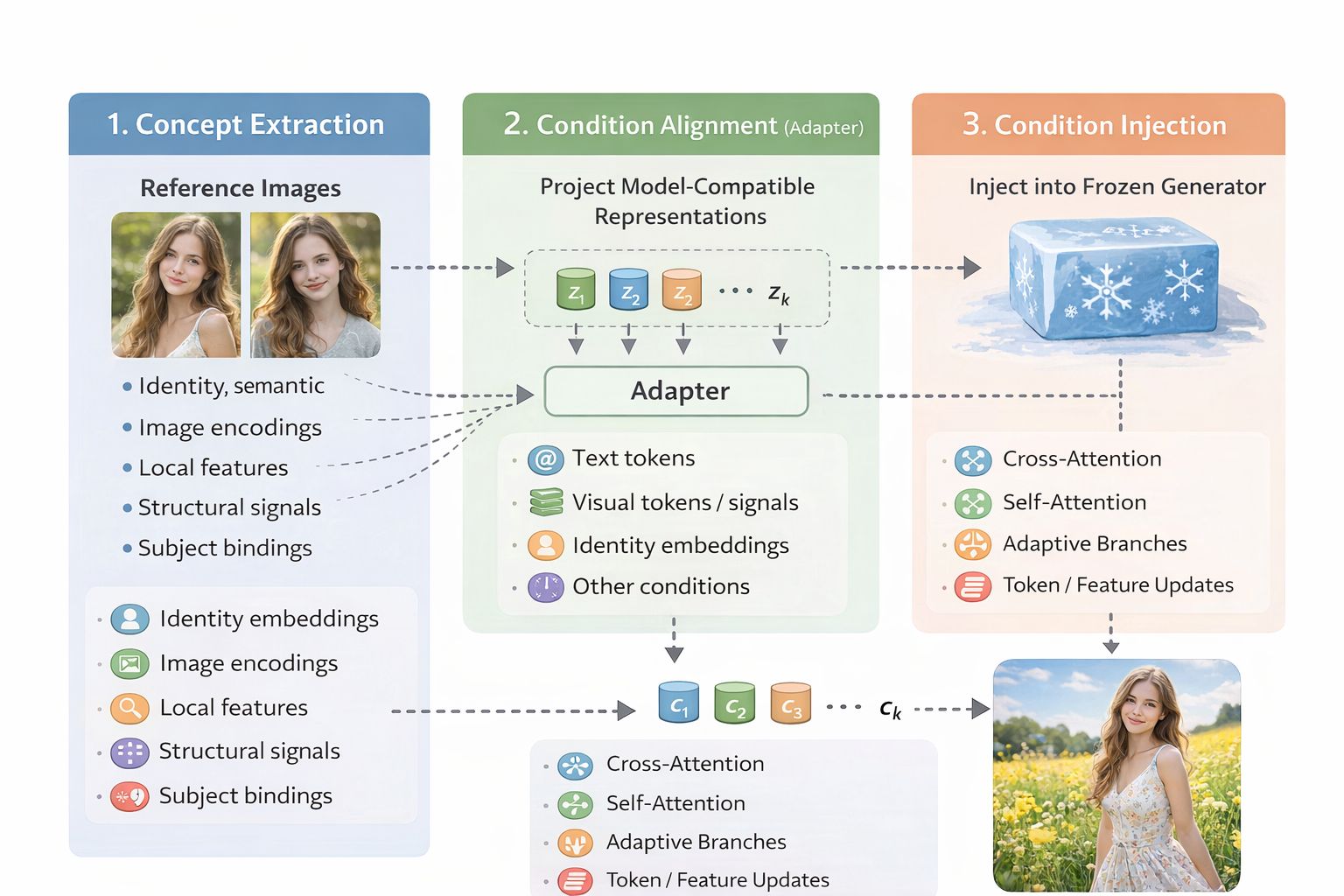
The three stages are not separate algorithm families. Rather, they form a common analytical lens. Almost every training-free personalization method contains all three components, but different methods place their main innovation at different stages.
11.1.1 Stage I: Concept Extraction
The first stage asks: What information should be extracted from the reference images?
A reference image contains many types of information. Some are concept-specific; others are incidental. For example, in a portrait reference image, the desired concept may be the person’s identity, while the background, lighting, camera angle, and clothing may or may not be relevant. In a product personalization task, shape, material, logo, and texture may matter more than global scene composition. In a multi-subject task, the method must also know which visual concept corresponds to which textual subject.
Therefore, training-free personalization methods often extract multiple types of visual signals:
Identity information. Identity information is especially important for human personalization. Face-oriented methods often rely on a face recognition model or identity encoder to obtain a compact representation of a person’s identity. This representation is usually more suitable for identity preservation than a generic image embedding, because generic image encoders may entangle identity with pose, style, clothing, or background.
Visual-semantic information. Visual-semantic information captures the global meaning of the reference image. This can include object category, style, color distribution, and overall appearance. CLIP-like image embeddings, DINO-like visual features, or BLIP-style multimodal representations are often used for this purpose. These features are useful for general subject personalization because they provide a high-level description of what the reference subject is.
Local appearance information. Local appearance information captures finer details that may be lost in a single global embedding. For example, a specific logo, facial detail, clothing pattern, accessory, or object texture may require patch-level or token-level features. This is why many methods do not rely only on a single pooled image embedding. They may also extract intermediate features, local visual tokens, or multi-layer representations.
Structural information. Structural information provides spatial control. Pose maps, depth maps, edge maps, masks, bounding boxes, landmarks, and layout signals do not necessarily describe “who” or “what” the subject is, but they help control “where” and “how” the subject appears. For identity-preserving generation, facial landmarks can stabilize pose and face geometry. For multi-object generation, masks and layout conditions can reduce subject confusion.
Subject-binding information. Subject-binding information becomes critical when multiple personalized concepts appear in the same prompt. If the prompt contains two people or two objects, the model must know which reference image corresponds to which textual phrase and which spatial region. Without such binding, attributes can leak from one subject to another, resulting in identity mixing or incorrect object assignment.
Thus, the extraction stage should not be understood as simply “encode the image.” It is better understood as: Decompose the reference images into the visual signals that are relevant to personalization.
Different methods choose different decompositions. Some extract only a global image embedding. Some combine global and local features. Some specialize in face identity. Some add landmarks or spatial maps. Some explicitly model multi-subject binding. These design choices largely determine the upper bound of concept fidelity.
11.1.2 Stage II: Condition Alignment
The second stage asks: How can the extracted visual signals be transformed into conditions that the generative model can understand?
The features produced by an image encoder are usually not directly compatible with a diffusion model. A CLIP image embedding, an ArcFace identity vector, a DINO patch feature, or a landmark map lives in its own representation space. The frozen generator, however, expects conditions in specific forms: text embeddings, cross-attention context tokens, timestep embeddings, residual features, ControlNet-like feature maps, AdaLN modulation vectors, or transformer tokens.
Therefore, an alignment module is needed. This module can be called an adapter, projector, resampler, mapper, ID encoder, or connector. Its role is analogous to the connector in vision-language models: it translates visual representations into the conditioning language of the generative backbone.
The aligned condition may take several forms:
Text-like tokens. The most direct strategy is to align the visual concept to the text embedding space. The reference image is encoded into one or several pseudo text tokens, which are then inserted into the prompt embedding sequence.
Conceptually, this is close to Textual Inversion, but with an important difference: Textual Inversion optimize a concept token for each new subject, while Text-space alignment predict a concept token from reference images at inference time.
The aligned condition has the form:
\[c = A(E_{\text{img}}(R)) \in \mathbb{R}^{m \times d_{\text{text}}},\]where $m$ is the number of pseudo tokens and \(d_{\text{text}}\) is the text embedding dimension.
This strategy is attractive because it preserves compatibility with the original text-conditioning pathway. The generated concept can be inserted into the prompt almost like a learned word. However, the text space is not designed to store all fine-grained visual details. As a result, text-space alignment may preserve global semantics but lose local appearance, texture, or identity-sensitive information.
Summary: Typical aligned outputs include: pseudo-word embeddings, subject tokens, text-compatible concept embeddings, layer-wise textual embeddings.
This route is especially useful when the method wants to remain close to the original prompt-conditioning mechanism.
Image-prompt tokens. A stronger alternative is to align the reference image into image-prompt tokens rather than text tokens. Instead of forcing visual information into the text embedding space, the method produces a set of visual tokens that can be consumed by the diffusion model through attention.
The aligned condition has the form:
\[c = A(E_{\text{img}}(R)) \in \mathbb{R}^{n \times d_{\text{attn}}},\]where $n$ is the number of image prompt tokens and \(d_{\text{attn}}\) matches the cross-attention hidden dimension.
This is the logic behind adapter-style personalization methods. The adapter may be a linear projector, an MLP, a resampler, or a Perceiver-style module. Its job is to compress or transform image encoder features into a fixed number of tokens suitable for the generator.
Summary: Common modules include: linear projection, MLP projector, Perceiver resampler, Q-Former-style query extractor, image prompt adapter, token compressor.
Compared with text-space alignment, image-prompt alignment usually has higher visual capacity because it does not need to squeeze the reference concept into a single word-like embedding. It can preserve richer appearance information and support multiple reference images. However, it also requires a dedicated injection mechanism, such as standard or decoupled cross-attention.
This strategy is central to methods such as IP-Adapter-like systems, where image conditions are represented as a separate token stream rather than being merged into the text prompt.
Identity embeddings. For human personalization, generic image features are often insufficient. A person’s identity is a fine-grained and highly discriminative concept. Therefore, many methods first extract an identity embedding using a face recognition model, then align this embedding to the generative model. The extracted identity feature may be:
\[z_{\text{id}} = E_{\text{face}}(R),\]where \(E_{\text{face}}\) can be an ArcFace-like or InsightFace-like encoder. However, this vector is trained for face recognition, not for image generation. It must be transformed into a form that can guide the diffusion model:
\[c_{\text{id}} = A_{\text{id}}(z_{\text{id}}).\]Summary: The aligned identity condition may become: identity tokens, ID-aware prompt embeddings, ID-specific cross-attention features, identity modulation vectors, identity-conditioned adapter features.
Identity-space alignment has a different objective from generic image-token alignment. It should preserve identity-discriminative information while suppressing nuisance factors such as lighting, pose, expression, background, and image style. If the alignment is too weak, the generated face does not resemble the reference subject. If it is too strong, the model may over-copy the reference image and lose editability.
This route is common in face personalization methods such as PhotoMaker, InstantID, PuLID, and related identity-preserving systems.
Spatial control features. Some reference signals are not primarily semantic or identity-based. They describe spatial structure: pose, layout, mask, depth, edge, segmentation, landmark, or bounding box information. These signals need a different alignment strategy.
Instead of mapping the condition into text tokens, the method maps it into spatial feature maps compatible with the denoising network:
\[c_{\text{spatial}} = A_{\text{spatial}}(S),\]where $S$ may be a pose map, landmark map, mask, depth map, or layout representation.
Summary: The aligned condition may be injected as: multi-scale residual features, ControlNet-style side-branch features, T2I-Adapter-style additive features, channel-concatenated inputs, region masks for localized attention.
Spatial-feature alignment is useful when personalization requires controllable geometry. For example, in human identity personalization, an identity embedding may tell the model “who” the subject is, while landmarks or pose maps tell it “how the face should be arranged.” In multi-subject personalization, masks or layouts can specify where each subject should appear.
This type of alignment is not mainly about concept appearance. It is about constraining the spatial organization of generation.
Attention-Space Alignment. Some methods align the visual concept directly to the attention mechanism of the generator. Instead of only producing tokens, the adapter may generate or modify the key-value representations used in cross-attention or self-attention.
A simplified cross-attention layer can be written as:
\[\mathrm{Attn}(Q, K, V) = \mathrm{softmax}\left(\frac{QK^\top}{\sqrt{d}}\right)V.\]In text-conditioned diffusion models, (Q) usually comes from noisy image features, while (K) and (V) come from text embeddings. Attention-space alignment modifies this interface by producing additional image-derived keys and values:
\[K_{\text{img}}, V_{\text{img}} = A(E_{\text{img}}(R)).\]The generator may then attend to both text and image conditions:
\[\mathrm{Attn}(Q, [K_{\text{text}}, K_{\text{img}}], [V_{\text{text}}, V_{\text{img}}]).\]Alternatively, text and image conditions may be handled by separate attention branches:
\[\mathrm{Attn}_{\text{text}}(Q, K_{\text{text}}, V_{\text{text}}) + \lambda \mathrm{Attn}_{\text{img}}(Q, K_{\text{img}}, V_{\text{img}}).\]This is the key idea behind decoupled cross-attention. The image condition is not forced to compete with text tokens in the same attention stream. Instead, it receives a dedicated attention path, and its strength can be controlled by a scale factor.
Attention-space alignment is powerful because personalization happens exactly at the interface where conditions influence denoising features. It also makes it easier to balance text controllability and reference-image fidelity.
Summary: Common forms include: additional cross-attention keys and values, decoupled image cross-attention, attention processor replacement, reference key-value injection, self-attention feature correspondence.
This alignment route is especially important for adapter-based and reference-based personalization methods.
Modulation-Space Alignment. In transformer-based diffusion models, especially DiT-like architectures, conditions are often injected through modulation rather than classical UNet cross-attention. The adapter may transform the visual concept into scale, shift, or gate parameters used in normalization and transformer blocks.
A simplified modulation form is:
\[h' = \gamma(c) \odot \mathrm{Norm}(h) + \beta(c),\]where $h$ is an intermediate hidden state, and \(\gamma(c)\), \(\beta(c)\) are condition-dependent modulation parameters.
In this case, condition alignment means mapping extracted visual features into modulation vectors:
\[(\gamma, \beta, g) = A(E_{\text{img}}(R)).\]Summary: The aligned condition may affect: AdaLN scale and shift, gating parameters, timestep-conditioning vectors, class-conditioning vectors, transformer block modulation.
This route becomes increasingly important in DiT-era personalization because the generator may rely less on UNet-style cross-attention and more on transformer token streams and adaptive normalization.
Compared with cross-attention alignment, modulation-space alignment tends to be more global. It changes how the block processes features rather than adding explicit reference tokens. This can be efficient, but it may be less interpretable and harder to localize.
Feature-Replacement / Token-Replacement Alignment. Some newer methods do not rely on a conventional adapter that outputs tokens or modulation vectors. Instead, they align the reference concept by identifying internal features or tokens that correspond to the subject and then replacing, copying, or blending them during generation.
The aligned condition is not necessarily a new embedding. It may be an internal feature state:
\[c = h_{\text{ref}}^{(\ell, t)},\]where \(h_{\text{ref}}^{(\ell, t)}\) denotes a reference feature or token at layer $\ell$ and timestep $t$. Then the generation process may use a replacement rule such as:
\[h_{\text{gen}}^{(\ell, t)} \leftarrow (1-\alpha_t)h_{\text{gen}}^{(\ell, t)} + \alpha_t h_{\text{ref}}^{(\ell, t)}.\]This type of alignment is common in reference-based editing and DiT-era token manipulation. The method aligns the reference and generation processes at the level of internal representations rather than external conditions.
Summary: Common forms include: reference feature copying, self-attention key-value replacement, denoising token replacement, subject token correspondence, timestep-adaptive feature blending.
This strategy can preserve strong visual consistency because it transfers internal features directly. However, it also risks over-constraining generation if the replacement is too strong or applied at the wrong timesteps.
Region / Binding Alignment. For multi-subject personalization, the key difficulty is not only representing each subject, but also aligning each subject with the correct text phrase and image region. Suppose there are multiple reference subjects:
\[R = \{R_1, R_2, \ldots, R_N\},\]and the prompt contains multiple subject mentions:
\[y = \{s_1, s_2, \ldots, s_N\}.\]The model must align:
\[R_i \leftrightarrow s_i \leftrightarrow \Omega_i,\]where $\Omega_i$ denotes the spatial region associated with subject $i$. This gives rise to region-aware or binding-aware alignment.
Summary: Common forms include: subject-specific tokens, subject-to-word assignment, subject masks, localized attention maps, layout constraints, region-specific image prompts.
Without this alignment, the model may mix identities, swap attributes, or apply one subject’s appearance to another subject. Therefore, multi-subject personalization often requires explicit mechanisms for subject binding and localized attention.
This alignment route is especially important for FastComposer-like methods and compositional personalization.
11.1.3 Stage III: Condition Injection
The third stage asks: Where and how should the aligned condition influence the frozen generator?
After concept extraction and condition alignment, the reference information has already been converted into a model-compatible form. It may be a pseudo text token, an image-prompt token sequence, an identity embedding, a spatial feature map, a modulation vector, or an internal reference feature. However, a compatible representation alone is not sufficient. The method must still decide where, when, how strongly, and under what spatial or semantic constraints this condition should act on the generator.
Condition injection is the operational stage of training-free personalization. While condition alignment determines the form of the reference signal, condition injection determines how that signal changes the denoising computation. The main design questions are:
Where is the condition injected? The first design choice is the location of injection. A condition can enter the generator at different depths and through different computational interfaces. At a high level, injection locations can be grouped into:
 input-level injection
 context-level injection
 block-level injection
 feature-level injection
 token-level injection
 output-level guidance
How is it fused? The second design choice is the fusion operator. Once a condition has reached a certain layer, the model must decide how to combine it with the current denoising features. Common fusion operators include:
   concatenation
   addition
   attention-based fusion
   affine modulation
   gated fusion
   feature blending
   feature replacement
   attention biasing
How strong is it? The third design choice is the strength of injection. In training-free personalization, this is especially important because the generator is frozen and the reference condition may not be perfectly aligned with the base model.
A generic strength-controlled injection can be written as:
\[h_{\ell,t}' = h_{\ell,t} + \lambda_{\ell,t} \Delta h_{\ell,t}(c),\]where \(\lambda_{\ell,t}\) controls the influence of the personalized condition at layer \(\ell\) and timestep $t$.
A small \(\lambda_{\ell,t}\) improves prompt editability but may weaken identity or subject fidelity. A large \(\lambda_{\ell,t}\) improves reference consistency but may cause over-copying, reduced diversity, or prompt neglect.
When is it injected? The fourth design choice is when to inject the condition during the denoising trajectory. Diffusion and flow-based generators gradually transform noise into a clean image. Different timesteps control different aspects of generation. Although the exact interpretation depends on the model and sampler, a useful intuition is:
 early timesteps:
     global layout, coarse structure, object placement

 middle timesteps:
     subject shape, identity, pose, semantic composition

 late timesteps:
     texture, color, local detail, refinement
Therefore, the same condition may have different effects at different timesteps. Injecting a strong identity condition too early may constrain the global composition. Injecting it too late may preserve texture but fail to establish correct identity. Injecting spatial structure early may help layout, while injecting local appearance details later may improve fine-grained consistency.
Which layers receive it? The fifth design choice is layer selection. A generative backbone contains multiple layers or blocks, each operating at different semantic and spatial levels. In UNet-based diffusion models, low-resolution blocks often encode global semantics and composition, while higher-resolution blocks refine local structure and texture. In DiT-based models, different transformer depths may also capture different levels of abstraction.
A layer-dependent injection rule can be written as:
\[h_{\ell,t}' = h_{\ell,t} + \lambda_{\ell}\Delta h_{\ell,t}(c).\]Different conditions may be injected into different layers:
 global image semantics:
     often injected into deeper or lower-resolution layers

 local texture and appearance:
     often injected into higher-resolution or later layers

 identity features:
     often require mid-level and high-level feature influence

 spatial structure:
     often injected across multiple resolutions

 region masks:
     often affect attention or feature maps at selected layers
Which regions does it affect? The sixth design choice is spatial selectivity. For single-subject personalization, global injection may be acceptable. But for multi-subject generation, editing, or localized personalization, the condition should only affect the relevant region. Otherwise, one subject’s identity, color, texture, or style may leak into another subject or into the background.
A spatially selective injection can be written as:
\[h_{\ell,t}' = h_{\ell,t} + m \odot \lambda \Delta h_{\ell,t}(c),\]where $m$ is a spatial mask or attention map. For multiple subjects:
\[h_{\ell,t}' = h_{\ell,t} + \sum_{i=1}^{N} m_i \odot \lambda_i \Delta h_{\ell,t}(c_i).\]Here, \(c_i\) is the condition for subject $i$, and $m_i$ specifies where this subject should influence the generation. Spatial selectivity can be implemented through:
 explicit masks
 bounding boxes
 layout maps
 segmentation maps
 localized attention
 region-specific cross-attention
 attention reweighting
 subject-token routing
How does it interact with text? The seventh design choice is condition balancing. Balanced with prompt semantics, separated through branches, or controlled by scales. Common balancing strategies include:
 separate text and image branches
 condition-specific scale factors
 layer-specific weighting
 timestep-specific weighting
 identity-only extraction
 spatial masking
 reference dropout during adapter training
 negative prompts or unconditional branches
How are multiple subjects routed? The eighth design choice is routing. When there are multiple personalized subjects, the generator must know which condition belongs to which subject mention and which image region. This is not guaranteed by simply concatenating all conditions.
This routing can be implemented through:
 subject-specific tokens
 localized attention masks
 region-conditioned attention
 layout-guided routing
 per-subject scaling
 attention constraints
 explicit subject-word binding
The goal is to ensure that each subject condition affects only its intended textual and spatial target. Without routing, multi-subject personalization can easily suffer from identity blending or attribute swapping.
How does the backbone affect injection? The final design choice is backbone specificity.
In UNet-based Stable Diffusion models, personalization often relies on:
 cross-attention processors
 residual feature injection
 ControlNet-style side branches
 multi-resolution feature maps
This is because the UNet architecture naturally exposes spatial feature maps and text cross-attention layers.
In DiT-style or MMDiT-style models, the situation is different. The generator operates over transformer token streams, and conditions may enter through:
 joint image-text attention
 token prepending
 token replacement
 AdaLN modulation
 gated transformer blocks
 internal feature routing
Therefore, injection mechanisms developed for UNet-based models may not transfer directly to DiT-based models. A DiT-era personalization method must consider how reference information flows through transformer tokens rather than only through cross-attention maps.
This architectural shift explains why newer personalization methods increasingly discuss token replacement, feature routing, joint attention, or modulation-based conditioning. In this sense, Stage III is also where the evolution from UNet-era personalization to DiT-era personalization becomes most visible.
11.1.4 Summary
Training-free personalization is not merely a faster version of DreamBooth. It represents a different way of thinking about concept injection. The new concept is no longer stored as a subject-specific parameter delta. Instead, it is extracted from reference images, transformed into model-compatible conditions, and injected into a frozen generator at inference time.
The unified pipeline can be summarized as:
\[R \xrightarrow{\text{extraction}} \{z_k\}_{k=1}^{K} \xrightarrow{\text{alignment}} \{c_k\}_{k=1}^{K} \xrightarrow{\text{injection}} G_\theta(x_t, t, y; c_1,\ldots,c_K),\]where $R$ denotes the reference images, $z_k$ denotes extracted visual signals, $c_k$ denotes aligned runtime conditions, and $G_\theta$ denotes the frozen generative model.
This framework highlights the three essential questions behind training-free personalization:
1. What concept information is extracted from the reference images?
2. How is this information aligned with the generator’s conditioning space?
3. Where and how is it injected into the denoising process?
The following sections use this lens to study major families of training-free personalization methods, moving from visual-to-token approaches, to image-prompt adapters, identity-centric systems, multi-subject binding methods, and finally DiT-era token or feature-level personalization. Below is a corrected table aligned with the three-stage framework.
| Method | Stage I: Concept Extraction | Stage II: Condition Alignment | Stage III: Condition Injection |
|---|---|---|---|
| ELITE | Extracts hierarchical/global visual features and local patch-level visual features from the reference image. | Uses a global mapping network to project hierarchical image features into multiple textual word embeddings, including one primary word and auxiliary words; uses a local mapping network to convert patch features into local textual feature embeddings. | Global textual embeddings are inserted into the prompt embedding stream; local mapped features are injected through additional cross-attention layers and fused with the global branch to recover fine details while preserving editability. |
| BLIP-Diffusion | Takes a subject image plus category text as input to a BLIP-2-style multimodal encoder; the frozen image encoder extracts visual features and a Q-Former-style multimodal encoder produces subject features. | Aligns the visual subject representation with the text space through BLIP-2-style multimodal representation learning, producing text-aligned subject prompt embeddings. | The subject representation is infixed / combined with the prompt embedding and used as an additional condition for the latent diffusion model. The core mechanism is subject-conditioned generation through text-compatible subject embeddings. |
| InstantBooth | Encodes an input image set using a Concept Encoder for global concept information and a Patch Encoder for local patch-level details. Both use CLIP image encoder backbones followed by learnable projections. | Maps the global concept feature into the textual embedding space; maps local patch tokens into a unified feature space. Adapter layers and concept-token normalization are used to balance identity preservation and language alignment. | Replaces the placeholder token embedding in the prompt with the global concept embedding; injects patch embeddings through additional adapter layers inserted inside the UNet transformer blocks, with gated control over visual-feature contribution. |
| IP-Adapter | Extracts image-prompt features using a CLIP image encoder from the reference image. | Projects image features into image prompt tokens compatible with the diffusion model’s attention dimensions. The image prompt is kept separate from the text prompt. | Injects image prompt tokens through decoupled cross-attention: the original text cross-attention is preserved, while a parallel image cross-attention branch is added and controlled by an image-prompt scale. |
| PhotoMaker | Takes an arbitrary number of human ID images and extracts per-image ID-related visual embeddings, together with the text prompt class-word context. | Builds a stacked ID embedding through an ID Encoder / FuseModule. The stacked embedding serves as a unified semantic representation of the input identity or identities. | Replaces the corresponding class-word embedding, such as “man” or “woman,” with the stacked ID embedding. No extra UNet branch is added; the original cross-attention layers consume the modified prompt embedding and integrate ID information. |
| InstantID | Extracts a face identity embedding from a single facial image and obtains facial landmark / keypoint information as weak spatial guidance. | Uses an Image Adapter to make the face embedding usable by the diffusion model, and an IdentityNet to combine strong semantic identity information with weak spatial facial-landmark conditions. | Injects identity through an adapter-style identity branch and uses IdentityNet as a ControlNet-like spatial control module. The final generation is steered by text prompt, face ID condition, and landmark condition together. |
| PuLID | Extracts ID features using both a face-recognition backbone and a CLIP image encoder. It uses the concatenated final-layer features for global ID information and CLIP multi-layer features for local ID information. | Maps concatenated face-recognition and CLIP features into global ID tokens with an MLP; maps CLIP multi-layer features into local ID tokens. The adapter is trained with a Lightning T2I branch, contrastive alignment loss, and accurate ID loss to reduce disturbance to the base model. | Embeds ID tokens using parallel cross-attention layers, following the IP-Adapter-style mechanism. The key difference is not the injection interface itself, but the training objective that teaches the ID insertion to preserve identity while minimally disrupting the original model behavior. |
| FastComposer | Extracts subject embeddings from reference subject images using an image encoder, especially for multiple human subjects. | Uses the extracted subject embeddings to augment generic word tokens in the text conditioning, such as replacing or enriching “person” tokens with subject-specific embeddings. | Uses subject-augmented text conditioning in the diffusion model. To mitigate identity blending, it trains with cross-attention localization supervision and uses delayed subject conditioning during denoising to balance identity preservation and editability. |
| InfiniteYou | Extracts identity features from the reference face for DiT / FLUX-based identity-preserved generation. | Projects identity features into a DiT-compatible identity feature set and feeds them into InfuseNet, a DiT-based identity injection network trained with a multi-stage strategy, including pretraining and SFT with SPMS data. | Injects identity features into the FLUX / DiT base model through residual connections between DiT blocks via InfuseNet. It explicitly avoids IPA-style attention modification for identity injection, in order to preserve text-image alignment and base model generation quality. |
| Personalize Anything | Obtains reference subject denoising tokens / subject tokens in a DiT-based generation process, often guided by masks or layouts when needed. | Does not use a conventional learned adapter. Alignment is achieved by selecting subject-relevant DiT tokens, preserving semantic token information while avoiding positional conflicts, and applying timestep-adaptive replacement rules plus patch perturbation. | Performs timestep-adaptive token replacement inside the DiT denoising process: early-stage replacement enforces subject consistency, later-stage multimodal attention / regularization improves flexibility. Patch perturbation is used to increase structural diversity; the same mechanism supports layout-guided, multi-subject, and mask-controlled personalization. |
11.2 Visual-to-Token Personalization
The first family of training-free personalization methods can be understood as visual-to-token personalization. Its central idea is simple: Instead of optimizing a new token embedding for each concept, learn a general encoder that predicts concept tokens from reference images.
This family is the closest training-free counterpart to Textual Inversion. Textual Inversion shows that a user-provided concept can be represented by one or a few learned “words” in the embedding space of a frozen text-to-image model. Once learned, these pseudo-words can be composed with ordinary prompts to place the concept in new scenes or styles. However, Textual Inversion still requires concept-specific optimization: every new subject needs its own learned embedding.
Visual-to-token methods replace this per-concept optimization with a learned image-to-condition encoder. Given a reference image or a small image set, the encoder predicts token-like representations that can be inserted into the diffusion model’s conditioning pathway. These predicted tokens may be text-compatible embeddings, subject prompt embeddings, global concept tokens, or a mixture of global tokens and local visual features. The important shift is that the concept is no longer stored as a newly optimized token; it is produced at inference time from the reference image.
In the three-stage framework introduced in Section 11.1, this family can be summarized as:
\[R \xrightarrow{\text{visual encoder}} z \xrightarrow{\text{token alignment}} c_{\text{token}} \xrightarrow{\text{prompt / attention injection}} G_\theta(x_t,t,y;c_{\text{token}}).\]Here, $R$ denotes the reference image or image set, $z$ denotes extracted visual features, \(c_{\text{token}}\) denotes the predicted token-like condition, and \(G_\theta\) is the frozen or mostly frozen text-to-image generator. In practice, the “token” may not always be a pure text token. ELITE, for example, combines global textual embeddings with local cross-attention features; InstantBooth combines a global textual embedding with local patch adapters. Nevertheless, these methods belong to the same design family because their core interface is still to translate visual concepts into token-like conditions that the text-conditioned generator can consume.
11.2.1 From Textual Inversion to Predicted Concept Tokens
Textual Inversion provides the conceptual starting point. It treats personalization as an inversion into the textual embedding space. Given a few images of a concept, it learns a pseudo-word embedding \(e_{S^*}\) such that prompts containing $S^*$ can reproduce the concept while remaining composable with natural language. Formally, if \(y(S^*)\) denotes a prompt containing the pseudo-token, the embedding is optimized so that the frozen denoising model reconstructs the reference concept:
\[e_{S^*}^{\star}= \arg\min_{e} \mathbb{E}_{x_0,\epsilon,t} \left[ \left\| \epsilon - \epsilon_\theta \bigl( x_t,t,\tau(y(e)) \bigr) \right\|_2^2 \right],\]where \(\tau(\cdot)\) denotes the text encoder, and only the pseudo-token embedding is optimized. The strength of this formulation is its compatibility: once \(S^*\) is learned, it behaves like a word and can be inserted into prompts such as “a watercolor painting of \(S^*\)” or “\(S^*\) on the beach.” The limitation is that each new concept requires a new optimization process.
Visual-to-token personalization keeps the same representational intuition but removes the per-concept optimization. Instead of solving for \(e_{S^*}\) separately for every new subject, it learns a generic function:
\[c_{\text{token}} = A(E_{\text{img}}(R)),\]where \(E_{\text{img}}\) extracts visual features from the reference image and $A$ maps these features into a token-like condition. During inference, a new concept is encoded by a single forward pass:
reference image(s) → image encoder → token-like concept condition → personalized generation
This turns personalization from an optimization problem into a recognition-and-conditioning problem. The method no longer asks, “Which token embedding should be learned for this subject?” It asks, “Can a general encoder predict a useful token representation for any new subject?”
This shift introduces a fundamental trade-off. Optimization-based methods can fit a specific subject more tightly because they adapt directly to that subject. Visual-to-token methods are much faster and more scalable, but their fidelity is bounded by the capacity of the encoder and the expressiveness of the target token space. A single text-compatible embedding may capture category, color, or rough identity, but it may lose fine-grained details such as texture, logos, facial subtleties, or object-specific geometry. For this reason, later visual-to-token methods often add local features, patch-level tokens, or adapter layers on top of the global token representation.
From the three-stage perspective, the common structure is:
| Stage | Role in visual-to-token personalization |
|---|---|
| Extraction | Extract global and/or local visual features from reference images. |
| Alignment | Map visual features into text-compatible tokens, subject tokens, or token-like conditions. |
| Injection | Insert these conditions into the prompt embedding, cross-attention context, or additional local attention/adapters. |
This section focuses on three representative methods: ELITE, BLIP-Diffusion, and InstantBooth. They all avoid test-time concept optimization, but they differ in how much information they try to encode into text-like tokens and how they compensate for the limited capacity of text space.
11.2.2 ELITE
ELITE, short for Encoding Visual Concepts into Textual Embeddings, is one of the clearest examples of the visual-to-token idea. Its motivation is that existing personalization methods can learn user-defined concepts through optimization, but this process is computationally expensive and must be repeated for every new concept. ELITE instead trains an encoder that maps a given concept image into textual embeddings, enabling fast customized generation.
The method is built around two complementary modules: Global mapping network, and Local mapping network
The global mapping network projects hierarchical visual features of the reference image into multiple textual word embeddings. The paper describes one primary word embedding and several auxiliary word embeddings. The primary word is intended to represent the editable concept, while the auxiliary words help account for irrelevant disturbances such as background or other visual factors. In other words, ELITE does not simply map an image to one pseudo-token; it maps visual features into a small set of token embeddings with different roles.
A simplified formulation is:
\[\{e_0,e_1,\ldots,e_m\} = A_{\text{global}} \bigl( E_{\text{img}}(R) \bigr),\]where $e_0$ is the primary concept embedding and \(e_1,\ldots,e_m\) are auxiliary embeddings. These embeddings live in the textual word embedding space and can be composed with natural language prompts. This is why ELITE is naturally connected to Textual Inversion: both operate in a text-embedding interface, but Textual Inversion optimizes a concept token, whereas ELITE predicts it.
However, ELITE also recognizes that the textual embedding space has limited visual capacity. A global token embedding can preserve semantic identity to some extent, but it may omit local details. To address this, ELITE introduces a local mapping network that encodes patch-level visual features into textual feature embeddings. These local features are injected through additional cross-attention layers and fused with the global branch. This local branch is designed to recover details that are hard to store in global word embeddings without sacrificing prompt editability.
From the extraction-alignment-injection viewpoint:
| Stage | ELITE |
|---|---|
| Extraction | Extracts hierarchical/global image features and local patch-level visual features from the reference image. |
| Alignment | Maps global features into multiple textual word embeddings; maps local patch features into local textual feature embeddings. |
| Injection | Inserts global textual embeddings into the prompt-conditioning path; injects local mapped features through additional cross-attention layers and fuses them with the global branch. |
The key insight of ELITE is that global text-like tokens provide editability, while local visual features provide detail fidelity. If the method relied only on a predicted pseudo-token, it would inherit the bottleneck of Textual Inversion: a word embedding is convenient but visually compressed. If it relied only on local features, it might preserve details but become less editable. ELITE’s architecture therefore reflects a balanced design: global mapping for semantic composability, local mapping for visual faithfulness.
This also reveals the broader limitation of visual-to-token personalization. The closer the condition is to the text space, the easier it is to compose with language, but the harder it is to preserve fine-grained appearance. ELITE’s local branch can be viewed as an early attempt to repair this compression loss without abandoning the text-token paradigm entirely.
11.2.3 BLIP-Diffusion
BLIP-Diffusion approaches visual-to-token personalization from a more explicitly multimodal perspective. Instead of treating personalization mainly as inversion into textual word embeddings, it introduces a pre-trained subject representation for subject-driven text-to-image generation. The model consumes both subject images and text prompts, and it uses a BLIP-2-style multimodal encoder to produce text-aligned subject representations.
The motivation is that most pre-trained text-to-image models are primarily text-conditioned. They do not natively support a subject image as a control input. If we want a diffusion model to generate new renditions of a reference subject, the subject image must be transformed into a representation that is compatible with the text-conditioned generation process. BLIP-Diffusion addresses this by adapting a BLIP-2 encoder to extract multimodal subject representation, which is then used together with the text prompt to guide generation.
A simplified pipeline is:
subject image + subject category text
        ↓
BLIP-2-style multimodal encoder
        ↓
text-aligned subject representation
        ↓
combined with generation prompt
        ↓
subject-driven diffusion generation
The subject category text is important because the model is not only asked to encode an image, but to encode the image as a specific subject category. For example, a reference image may contain a dog, a backpack, or a toy; the category label helps the multimodal encoder focus on the subject representation rather than arbitrary image content. This makes the extracted representation more suitable for subject-driven generation.
In the alignment stage, BLIP-Diffusion produces a subject representation aligned with the text space. The paper describes pre-training the multimodal encoder following BLIP-2 to produce visual representations aligned with text, followed by a subject representation learning task that enables the diffusion model to use this representation for new subject renditions.
From the extraction-alignment-injection viewpoint:
| Stage | BLIP-Diffusion |
|---|---|
| Extraction | Uses subject image and category text as input to a BLIP-2-style multimodal encoder. |
| Alignment | Produces a text-aligned subject representation through multimodal pre-training and subject representation learning. |
| Injection | Combines subject prompt embeddings with text prompt embeddings to guide the diffusion model. |
Compared with ELITE, BLIP-Diffusion is less like “predict a pseudo-word from an image” and more like “pre-train a generic subject representation interface.” This makes it conceptually closer to modern vision-language connectors. The subject representation is not merely a static word embedding; it is a multimodal representation learned to be usable by a diffusion generator.
This difference matters. ELITE is organized around the text embedding space and repairs its limitations with local mapping. BLIP-Diffusion starts from a multimodal encoder and trains the diffusion model to use the resulting subject representation. As a result, it can serve as a more general subject-driven generation system and can be combined with other control methods such as ControlNet or attention-based editing. The BLIP-Diffusion paper explicitly demonstrates combinations with ControlNet and prompt-to-prompt-style editing, suggesting that subject representation can coexist with additional structural or editing controls.
The limitation is that the method depends heavily on the quality of the pre-trained subject representation. If the multimodal encoder fails to isolate the target subject, or if the category text is ambiguous, the subject representation may include background, pose, or context artifacts. Moreover, because the representation is generic, it may not reach the same fidelity as subject-specific optimization in difficult cases. Its advantage is speed and scalability: new subjects can be handled without lengthy test-time fine-tuning.
11.2.4 InstantBooth
InstantBooth is another training-free personalization method, but it makes the limitation of pure token prediction especially explicit. The paper’s goal is personalized text-to-image generation without test-time fine-tuning. It first maps the input image set into a global concept embedding in the textual embedding space, but it also introduces local adapter layers to preserve fine details.
The key observation is that a global textual embedding alone may be insufficient for identity or concept preservation. If all reference information is compressed into a single global token, the model may capture the rough category or appearance but lose the detailed identity cues needed for faithful personalization. InstantBooth therefore uses two complementary components: A global concept encoder, and Local visual adapters / patch-level representations
The global concept encoder maps the reference images into a textual embedding. This embedding is integrated into the original prompt embeddings to enhance the corresponding word token, such as “person” in the prompt. This makes the new concept accessible through the same broad interface as text-conditioned generation: the model still receives a prompt embedding sequence, but one part of that sequence is enhanced by the visual concept.
A simplified formulation is:
\[e_{\text{concept}} = A_{\text{global}} \left( E_{\text{img}}(R_1,\ldots,R_n) \right),\]and this concept embedding is inserted into or used to enhance the class-word embedding in the prompt. For example, in a prompt such as “a person wearing sunglasses,” the visual embedding may enhance the representation of “person,” making it refer to the person in the reference images rather than a generic person.
However, InstantBooth does not rely only on this global embedding. To preserve fine-grained details, it introduces rich visual feature representations through adapter layers added to the pre-trained model. In the original paper description, the method uses a concept encoder to map image sets into global textual embedding space and introduces adapter layers to retain fine details of the input concept.
From the extraction-alignment-injection viewpoint:
| Stage | InstantBooth |
|---|---|
| Extraction | Extracts global concept information from the input image set and local visual details from image features. |
| Alignment | Maps the global concept into the textual embedding space; maps local visual information into adapter-consumable features. |
| Injection | Enhances the corresponding prompt word with the global concept embedding and injects local visual features through adapter layers in the generative model. |
InstantBooth is therefore best understood as a hybrid visual-to-token method. Its global branch follows the visual-to-token paradigm: image set to concept embedding to prompt conditioning. Its local branch acknowledges that textual embedding space is too narrow for complete personalization. This makes it conceptually similar to ELITE: both methods combine global token-like alignment with local feature compensation. The difference is architectural: ELITE uses global and local mapping networks, with local features injected through additional cross-attention layers; InstantBooth uses a concept encoder plus adapter layers to retain detailed identity or concept information.
The strength of InstantBooth is speed and convenience. Since it does not require test-time fine-tuning, it can personalize unseen concepts with a forward pass through the learned components. Its weakness is the same structural bottleneck shared by this family: the more it relies on predicted global tokens, the more it risks losing subtle identity details; the more it relies on local adapters, the more it begins to resemble image-prompt adapter methods rather than pure visual-to-token personalization.
11.2.5 Strengths and Limitations
Visual-to-token personalization occupies an important middle ground between optimization-based concept injection and more explicit image-adapter methods. Its strength is that it preserves the language-like interface of text-to-image models. A reference concept becomes a token-like condition that can be composed with natural language. This makes the method intuitive: users can provide reference images and then prompt the model as if the concept had become part of the vocabulary.
The main strengths are:
1. No concept-specific optimization at inference time.
2. Strong compatibility with existing text-conditioned diffusion models.
3. Natural composability with prompts.
4. Lower storage overhead than per-concept LoRA or DreamBooth models.
5. A clear bridge from Textual Inversion to training-free personalization.
Compared with Textual Inversion, the major advantage is speed. The method does not need to optimize a new embedding for every subject. Compared with DreamBooth-style full or partial fine-tuning, it avoids storing separate model deltas for every concept. Compared with pure image-prompt adapters, it keeps a closer connection to the text-conditioning interface, which can make prompt composition more direct.
However, the family also has important limitations.
First, textual embedding space is a bottleneck. A word embedding was not designed to store all visual details of a unique object or identity. It may encode semantic category and coarse appearance, but it can lose fine-grained texture, geometry, logo details, or subtle facial identity. This is exactly why ELITE adds local mapping and InstantBooth adds adapter layers. The moment a method needs local patches, cross-attention feature injection, or additional adapters, it is implicitly admitting that global token prediction alone is insufficient.
Second, visual-to-token alignment may entangle subject and context. A reference image contains background, lighting, pose, camera view, style, and other incidental attributes. If the encoder maps all of this into the concept token, the generated results may over-preserve irrelevant aspects of the reference image. ELITE’s auxiliary words are partly motivated by this issue: they help separate the editable primary concept from irrelevant disturbances such as background.
Third, generalization is bounded by the training distribution. Since the encoder is trained once and reused for unseen concepts, it must learn a general rule for extracting and representing concepts. If a new subject falls outside the training distribution, the predicted token may be weak or inaccurate. Optimization-based methods can still adapt to such a subject by directly fitting the reference images; training-free encoders cannot adapt unless additional fine-tuning is allowed.
Fourth, identity fidelity can be weaker than face-specialized methods. For human personalization, generic visual-to-token representations may not preserve identity as reliably as methods that use face recognition embeddings, landmarks, or ID-specific adapters. This is why Section 11.4 treats identity-embedding-centric personalization as a separate family. Human identity is not merely a generic visual concept; it requires highly discriminative and carefully aligned features.
Fifth, multi-subject binding remains difficult. If several predicted concept tokens are inserted into one prompt, the model may confuse which token corresponds to which subject or which attribute belongs to which subject. Visual-to-token methods alone do not automatically solve subject binding, attribute leakage, or identity mixing. This motivates binding-aware methods such as FastComposer, discussed later in Section 11.5.
A concise comparison is:
| Method family | Main interface | Main advantage | Main limitation |
|---|---|---|---|
| Textual Inversion | optimized pseudo-token | simple and composable | requires per-concept optimization |
| Visual-to-token personalization | predicted concept tokens | fast and prompt-compatible | token space limits visual fidelity |
| Image-prompt adapters | visual token branch | richer image conditioning | needs extra attention/interface design |
| Identity-centric methods | ID embeddings / ID tokens | stronger human identity | often specialized to faces or persons |
| Binding-aware methods | subject-region routing | better multi-subject composition | requires explicit binding or localization |
Overall, visual-to-token personalization should be viewed as the first major training-free response to Textual Inversion. It preserves the appealing idea that a new concept can be represented as something token-like and composed with language, but it replaces per-concept optimization with a learned encoder. Its historical and conceptual importance lies in this transition:
learn a token for each concept
        ↓
predict a token from reference images
        ↓
augment token prediction with local features and adapters
This transition also reveals why the field gradually moves beyond pure visual-to-token methods. Once the community recognizes that text-like tokens alone cannot faithfully carry all visual details, the next natural step is to introduce dedicated image-prompt branches, identity-specific embeddings, spatial controls, and DiT-level token or feature manipulation. These later families do not reject visual-to-token personalization; rather, they extend it by increasing the capacity, specificity, and controllability of runtime concept conditioning.
11.3 Image-Prompt Adapter Personalization
The second family of training-free personalization methods can be understood as image-prompt adapter personalization. It addresses a limitation that becomes clear in visual-to-token methods: if a reference image is forced into the text embedding space, much of its visual information may be compressed away. A pseudo text token is convenient for prompt composition, but it is not necessarily the best container for appearance, texture, shape, style, or identity-relevant details.
Image-prompt adapter methods therefore make a different design choice: Instead of translating the reference image into a text-like token, preserve it as an image-derived condition and inject it through a dedicated visual conditioning branch.
This shift changes the role of the reference image. In visual-to-token methods, the image is often treated as something that should be converted into the language interface of the diffusion model. In image-prompt adapter methods, the image is treated as a new type of prompt, parallel to the text prompt. The text prompt still controls semantics, scene, action, style, and edit instructions; the image prompt provides visual appearance, subject cues, or style information.
The generic pipeline is:
\[R \xrightarrow{\text{image encoder}} z_{\text{img}} \xrightarrow{\text{image adapter}} c_{\text{img}} \xrightarrow{\text{visual-condition injection}} G_\theta(x_t,t,y;c_{\text{img}}).\]Here, $R$ denotes the reference image, \(z_{\text{img}}\) denotes image features extracted by a frozen image encoder, \(c_{\text{img}}\) denotes image prompt tokens produced by a trainable adapter, and \(G_\theta\) is the frozen text-to-image diffusion model.
The key difference from Section 11.2 is the target alignment space:
Visual-to-token personalization:
    reference image → text-compatible concept token

Image-prompt adapter personalization:
    reference image → image prompt tokens → dedicated visual conditioning branch
This distinction is important. The image prompt does not need to behave like a word. It can be a sequence of visual tokens that directly participate in attention. This gives the method higher visual capacity and makes it easier to preserve image-level appearance. At the same time, because the image condition is separated from the text condition, the model can maintain stronger language controllability. In the three-stage framework:
| Stage | Role in image-prompt adapter personalization |
|---|---|
| Extraction | Extract visual features from the reference image, usually through a frozen image encoder. |
| Alignment | Project visual features into image prompt tokens compatible with the diffusion model’s attention dimensions. |
| Injection | Inject image prompt tokens through a separate or decoupled attention branch, while preserving the original text-conditioning pathway. |
The representative method in this family is IP-Adapter. Although later methods extend the idea to faces, identity embeddings, style control, and stronger vision encoders, the essential architectural principle is already clear in IP-Adapter: keep the base text-to-image model frozen, train a lightweight image adapter, and inject visual prompts through decoupled cross-attention.
11.3.1 From Text Tokens to Image Prompt Tokens
Text-to-image diffusion models are usually trained with text prompts as their primary condition. In Stable Diffusion-style architectures, the prompt is encoded by a text encoder and then injected into the UNet through cross-attention. At a cross-attention layer, the noisy image feature provides the query, while the text embeddings provide keys and values:
\[\mathrm{Attn}(Q, K_{\text{text}}, V_{\text{text}}) = \mathrm{softmax} \left( \frac{QK_{\text{text}}^\top}{\sqrt{d}} \right) V_{\text{text}}.\]The success of text-conditioned diffusion models shows that cross-attention is a powerful interface for controlling generation. However, it also reveals a constraint: if every new condition must be expressed as text, then non-linguistic visual information must be squeezed into a space originally designed for language.
Visual-to-token methods follow this text interface. They ask whether a reference image can be converted into a pseudo-word or subject token. Image-prompt adapter methods ask a different question: If text can act as a prompt through cross-attention, can an image also act as a prompt through a parallel attention interface?
This leads to the idea of image prompt tokens. An image prompt token is not a word embedding. It is a visual condition derived from the reference image and projected into a dimension that the diffusion model can attend to.
The transformation can be written as:
\[C_{\text{img}} = A_{\text{img}}(z_{\text{img}}) = A_{\text{img}}(E_{\text{img}}(R)),\]where \(E_{\text{img}}\) is a frozen image encoder, \(A_{\text{img}}\) is a trainable adapter, and
\[C_{\text{img}} \in \mathbb{R}^{n \times d}\]is a sequence of $n$ image prompt tokens with hidden dimension $d$. These tokens are then used as additional visual conditions inside the diffusion model.
This design has several advantages over pure text-token conversion.
First, image prompt tokens have higher visual capacity. A single pseudo-word embedding must compress the reference concept into one vector. An image prompt can be a sequence of tokens, allowing it to carry richer appearance information.
Second, image prompt tokens do not need to imitate natural language. They can remain closer to the visual feature space, which may better preserve color, texture, identity cues, shape, or style.
Third, image prompt tokens can be injected separately from text tokens. This separation is crucial because text and image conditions often play different roles. The text prompt specifies what should be generated; the image prompt specifies what the generated subject or style should resemble.
A useful comparison is:
Text prompt:
    controls semantic intent, scene, action, style words, compositional instructions

Image prompt:
    controls visual appearance, subject reference, style reference, or identity-like cues
If both conditions are merged naively into a single token sequence, they may compete for attention. The model may over-follow the image and ignore the prompt, or over-follow the prompt and lose reference fidelity. Image-prompt adapter methods therefore need not only a visual adapter, but also a careful injection design. This is where decoupled cross-attention becomes important.
11.3.2 IP-Adapter
IP-Adapter, short for Image Prompt Adapter, is the canonical method in this family. Its goal is to enable image-prompt capability for pre-trained text-to-image diffusion models without fine-tuning the entire model. The design is intentionally lightweight: the base diffusion model is frozen, the image encoder is typically frozen, and only a small adapter module is trained.
The method can be summarized as:
reference image
      ↓
frozen image encoder
      ↓
image feature
      ↓
trainable image projection module
      ↓
image prompt tokens
      ↓
decoupled cross-attention in the frozen diffusion model
This gives IP-Adapter two important properties.
First, it is parameter-efficient. The original diffusion model does not need to be retrained. The learned module is small relative to the full model.
Second, it is training-free for new concepts. Once the adapter is trained, a new reference image can be used directly at inference time. The user does not need to optimize a new token embedding, LoRA module, or concept-specific UNet delta.
From the extraction-alignment-injection framework:
| Stage | IP-Adapter |
|---|---|
| Extraction | Extracts image features from the reference image using a frozen image encoder. |
| Alignment | Projects image features into image prompt tokens compatible with the diffusion model’s cross-attention dimensions. |
| Injection | Injects image prompt tokens through decoupled cross-attention, while preserving the original text cross-attention branch. |
The defining architectural contribution of IP-Adapter is not merely that it uses image features. Many methods can extract image features. The key is decoupled cross-attention.
In the original text-to-image model, a cross-attention layer computes:
\[Z_{\text{text}} = \mathrm{Attn}(Q, K_{\text{text}}, V_{\text{text}}),\]where $Q$ comes from the noisy latent feature and \(K_{\text{text}}, V_{\text{text}}\) come from text embeddings.
A naive image-conditioning design might concatenate text and image tokens:
\[Z = \mathrm{Attn} \left( Q, [K_{\text{text}},K_{\text{img}}], [V_{\text{text}},V_{\text{img}}] \right).\]This is simple, but it entangles text and image conditions in the same attention operation. Text tokens and image tokens compete directly. The model must decide within a single softmax distribution whether to attend to text or image. This can weaken either prompt controllability or image fidelity.
IP-Adapter instead uses a decoupled formulation:
\[Z = Z_{\text{text}} + \lambda Z_{\text{img}}.\]where
\[\begin{aligned} Z_{\text{text}} & = \mathrm{Attn}(Q, K_{\text{text}}, V_{\text{text}}), \\[10pt] Z_{\text{img}} & = \mathrm{Attn}(Q, K_{\text{img}}, V_{\text{img}}), \end{aligned}\]Here, \(Z_{\text{text}}\) preserves the original text-conditioning pathway, while \(Z_{\text{img}}\) introduces image-prompt information through a separate attention branch. The coefficient $\lambda$ controls the strength of the image prompt.
This design has an important interpretation: Text and image are not forced into a single conditioning stream. They are treated as two complementary prompts with separate attention paths.
This separation makes IP-Adapter highly modular. It can be added to a pre-trained diffusion model without replacing the original text-conditioning mechanism. It can also be combined with other controls, such as LoRA, ControlNet, style adapters, or prompt engineering, because the base model remains largely intact.
The image projection module is also important. The output of an image encoder is not directly usable by the UNet cross-attention layers. The adapter maps the image feature into a set of image prompt tokens with the correct hidden dimension. In a simplified form:
\[C_{\text{img}} = A_{\text{proj}} \left( E_{\text{img}}(R) \right).\]Then image keys and values are produced from these tokens:
\[K_{\text{img}} = W_K^{\text{img}} C_{\text{img}}, \qquad V_{\text{img}} = W_V^{\text{img}} C_{\text{img}}.\]The trainable components include the image projection module and the parameters needed for the image cross-attention branch. The original text cross-attention pathway is preserved. The result is a simple but powerful image-conditioned personalization mechanism. It does not learn a concept-specific embedding; it learns a general way to make reference images usable as prompts.
11.3.3 Strengths and Limitations
Image-prompt adapter personalization has become influential because it offers a strong balance of efficiency, compatibility, and visual fidelity. It does not require per-concept fine-tuning, but it provides more visual capacity than pure text-token prediction. Its main strengths are:
- No test-time optimization for each new concept.
- Higher visual capacity than a single pseudo text token.
- Strong compatibility with existing text-to-image diffusion models.
- Modular integration with other controls such as LoRA and ControlNet.
- Adjustable text-image trade-off through image-prompt scale.
- Preservation of the original text-conditioning pathway.
However, image-prompt adapter personalization also has limitations.
- Image Prompts Are Not Always Identity-Preserving
- The Image Condition May Overpower the Text Prompt
- Global Image Prompts Can Introduce Unwanted Context
- Multi-Subject Binding Remains Difficult
- The Adapter Is General but Not Subject-Optimized
- Injection Is Architecture-Dependent
11.4 Identity-Embedding-Centric Human Personalization
Human identity personalization deserves a separate method family. Although it can be viewed as a special case of subject-driven generation, face identity is not just another visual concept like “a specific backpack,” “a particular dog,” or “a toy figure.” Human identity requires much finer semantic discrimination. Small changes in facial geometry, eye shape, skin texture, hairstyle, age cues, or expression can make the generated person look like someone else. At the same time, a useful personalization system should not simply copy the reference photo. It should preserve identity while allowing the text prompt to change pose, expression, clothing, style, camera view, age, accessories, and background.
This creates a stricter objective than generic image-prompt personalization. Therefore, identity-centric methods usually introduce specialized identity representations rather than relying only on generic image features. A CLIP image embedding may capture broad semantics, style, color, and composition, but it is not primarily trained for identity verification. InstantID explicitly argues that CLIP features are weakly aligned for high-fidelity ID preservation and instead uses a face model to extract strong identity features. PuLID similarly observes that tuning-free ID methods often use an encoder such as CLIP or a face-recognition backbone, but the main difficulty is to insert ID information without disrupting the original text-to-image model’s behavior.
From the three-stage perspective introduced in Section 11.1, identity-centric personalization can be summarized as:
\[R_{\text{id}} \xrightarrow{\text{ID extraction}} z_{\text{id}} \xrightarrow{\text{ID alignment}} c_{\text{id}} \xrightarrow{\text{identity injection}} G_\theta(x_t,t,y;c_{\text{id}},c_{\text{spatial}}).\]Here, \(R_{\text{id}}\) denotes one or more reference identity images, \(z_{\text{id}}\) is the extracted identity representation, \(c_{\text{id}}\) is the aligned identity condition, and \(c_{\text{spatial}}\) may optionally denote landmarks, keypoints, masks, or control images. The generator \(G_\theta\) is typically kept frozen at inference time; the new identity is not learned through per-person fine-tuning but is provided as a runtime condition.
The representative methods in this section are PhotoMaker, InstantID, PuLID, and InfiniteYou. They share the same high-level goal, but they make different design choices:
PhotoMaker:
    represent identity as a stacked ID embedding inserted into the text-conditioning stream.

InstantID:
    combine a face-identity embedding with an image adapter and IdentityNet for strong semantic and weak spatial identity control.

PuLID:
    use ID insertion with contrastive alignment and accurate ID loss to reduce disturbance to the original model while preserving identity.

InfiniteYou:
    move identity-preserved generation to DiT / FLUX-style backbones using InfuseNet residual injection rather than IPA-style attention modification.
The main axis of comparison is no longer just “how similar is the generated face?” A strong identity method must balance three goals: identity fidelity, prompt editability, and minimal disturbance to the base model.
A method that only maximizes identity similarity may over-copy the reference image or degrade prompt following. A method that only preserves editability may fail to maintain the person’s identity. A method that injects identity too aggressively may damage the base model’s style, composition, aesthetics, or text-image alignment. This fidelity-editability-disturbance trade-off is the central theme of identity-embedding-centric personalization.
11.4.1 Why Face Identity Requires Specialized Representations
Generic subject personalization usually aims to preserve a subject’s appearance. For example, if the reference subject is a dog, a bag, or a toy, the model should preserve its color, shape, texture, and category-specific details. Human identity personalization is more difficult because identity is a highly discriminative semantic concept. Two people may share similar hair, clothing, skin tone, or pose, but still have different identities. Conversely, the same person may appear under different lighting, age, expression, hairstyle, accessories, and viewpoints while still being recognized as the same identity.
This means that a useful identity representation must be both stable and editable:
stable:
    it should preserve identity across pose, expression, style, and lighting changes.

editable:
    it should not lock the generated image to the reference photo’s clothing, background, pose, or expression.
This is why face recognition embeddings are attractive. Unlike generic image embeddings, face recognition embeddings are trained to distinguish identities while suppressing many nuisance variations. In the context of diffusion personalization, such embeddings provide a more identity-specific signal than ordinary visual features. InstantID explicitly replaces CLIP-style generic visual prompting with a pre-trained face model to extract face ID embeddings, because CLIP features tend to capture broad and ambiguous semantics such as composition, style, and colors, which are insufficient for precise ID preservation.
However, a face recognition embedding alone is not enough. Face recognition models are trained for verification or retrieval, not for generative conditioning. Their feature space is not automatically compatible with the conditioning space of a diffusion model. Therefore, identity-centric methods need an alignment module that converts a recognition feature into a generative condition. Depending on the method, the aligned identity condition may become:
a text-compatible ID embedding,
an ID token sequence,
an image-prompt-like identity condition,
a cross-attention condition,
a ControlNet-like spatial condition,
or a residual injection signal for DiT blocks.
A second challenge is that identity must often be combined with weak spatial control. A face embedding may tell the model “who this person is,” but it does not fully specify where the face should be, how it should be oriented, or how the facial geometry should be arranged. InstantID addresses this by combining strong semantic identity conditions with weak spatial facial landmark conditions. InfiniteYou similarly allows an optional control image, such as a five-facial-keypoint image, to control the generation position of the subject.
A third challenge is model disturbance. If identity information is inserted too strongly or through an inappropriate interface, the model may lose its original text-following ability, style control, or generation quality. PuLID makes this problem central: it argues that ID insertion should alter only ID-related aspects while keeping ID-irrelevant elements such as background, lighting, composition, and style as consistent as possible with the original model behavior.
Thus, identity-centric personalization is not merely “use a better image encoder.” It requires a coordinated design:
1. Extract identity-specific information.
2. Align it to the generator’s conditioning space.
3. Inject it strongly enough to preserve identity.
4. Keep it selective enough to preserve prompt editability.
5. Avoid disrupting the base model’s original behavior.
This explains why identity-centric methods evolved beyond general visual-to-token and image-prompt adapter methods. Human identity requires a more specialized concept representation, a more careful injection policy, and a more explicit treatment of fidelity-editability trade-offs.
11.4.2 PhotoMaker
PhotoMaker is an efficient training-free human personalization method based on stacked ID embedding. Its goal is to generate realistic human photos that retain the characteristics of one or more input ID images while allowing the prompt to change content or attributes. Unlike DreamBooth or LoRA-style methods, PhotoMaker does not require per-ID fine-tuning at inference time; it constructs an ID representation from input images in a single forward process.
The key idea is to represent identity not by a single image embedding, but by a stack of ID embeddings extracted from multiple input ID images. Each subpart of the stacked embedding corresponds to one input image. This allows the method to capture more comprehensive ID information than a single reference image. The paper explicitly states that PhotoMaker stacks the encodings of multiple input ID images at the semantic level to construct a unified ID representation.
Stage I: Concept Extraction. PhotoMaker uses a CLIP image encoder to extract image embeddings from the input ID images. Before feeding each image into the image encoder, the method masks non-relevant regions by filling areas other than the body part of the specific ID with random noise, reducing the influence of other identities and background. It also fine-tunes part of the image encoder’s transformer layers and introduces learnable projection layers so that the extracted image embeddings can be injected into the same dimensional space as the text embedding.
Given $N$ input ID images \(\{X_i\}_{i=1}^{N}\), PhotoMaker extracts projected image embeddings:
\[\{e_i \in \mathbb{R}^{D}\}_{i=1}^{N}.\]Each \(e_i\) corresponds to ID information from one input image. The important point is that PhotoMaker does not treat the identity as a single fixed vector. It keeps multiple image-level ID embeddings and later concatenates them into a stacked representation.
Stage II: Condition Alignment. PhotoMaker aligns image embeddings with the text-conditioning space. For a given prompt, it extracts the text embedding and identifies the corresponding class word, such as “man” or “woman.” The feature vector at the class-word position is fused with each image embedding using two MLP layers. This fusion produces a set of fused ID embeddings: \(\{\hat{e}_i\}_{i=1}^{N}\).
The method then concatenates these fused embeddings along the sequence-length dimension to form the stacked ID embedding:
\[s^\ast = \mathrm{Concat}([\hat{e}_1,\ldots,\hat{e}_N]), \qquad s^\ast \in \mathbb{R}^{N \times D}.\]This design is important because the class word provides semantic context. The same identity image can be interpreted differently depending on whether the prompt class word is “man,” “woman,” “boy,” “girl,” or another human-related category. PhotoMaker uses this fusion to improve semantic controllability, including changes such as age and gender through prompt wording.
Stage III: Condition Injection. PhotoMaker injects the stacked ID embedding by replacing the feature vector at the class-word position in the original text embedding with the stacked ID embedding. The updated text embedding is then consumed by the original cross-attention layers of the diffusion model:
\[Q = W_Q \phi(z_t), \qquad K = W_K t^\ast, \qquad V = W_V t^\ast,\]where \(t^\ast\) is the updated text embedding containing the stacked ID embedding. The cross-attention mechanism adaptively integrates the ID information contained in the stacked embedding.
A critical correction is that PhotoMaker is not an IP-Adapter-style method that adds a separate image cross-attention branch. The paper emphasizes that the stacked ID embedding is integrated by replacing the class word in the text embedding, allowing the original cross-attention mechanism to merge ID information. However, to help the diffusion model better perceive the ID information in the stacked embedding, PhotoMaker additionally trains LoRA residuals for the attention matrices.
aker is its simplicity and efficiency. It can accept multiple ID images, produce a richer ID representation than a single embedding, and keep the inference process fast. It also supports interesting identity mixing: although the training uses multiple images of the same ID, the authors report that different IDs can be used at inference time to construct a mixed stacked ID embedding.
Its limitation is that the identity condition is still routed primarily through the text-conditioning stream. This makes PhotoMaker efficient and prompt-compatible, but it also means that very fine-grained identity control may be less direct than methods that use face-recognition embeddings, landmark controls, or dedicated identity branches. PhotoMaker is therefore best viewed as a semantic ID embedding method rather than a general image adapter or ControlNet-style identity controller.
11.4.3 InstantID
InstantID is a zero-shot identity-preserving generation method designed to use only a single facial image while maintaining high fidelity and compatibility with pre-trained text-to-image diffusion models. The method is explicitly motivated by the limitations of both tuning-based methods and earlier ID embedding methods: per-subject fine-tuning is expensive, while existing single-forward ID methods may lack compatibility with community models or fail to maintain high face fidelity.
InstantID introduces two core designs:
1. An Image Adapter that uses ID embedding as an image prompt.
2. IdentityNet, which imposes strong semantic and weak spatial identity conditions.
The paper states that InstantID uses a plug-and-play module that handles image personalization in various styles using only one facial image. It designs IdentityNet by imposing strong semantic and weak spatial conditions, integrating facial and landmark images with textual prompts to steer generation.
Stage I: Concept Extraction. InstantID extracts a face ID embedding from a single reference facial image using a pre-trained face model. This is a deliberate departure from methods that rely on CLIP image embeddings. The authors argue that CLIP features capture broad and ambiguous semantics, such as composition, style, and color, but are not sufficient for precise identity preservation. A face model provides stronger identity-specific features.
In addition to the identity embedding, InstantID uses facial landmark information as weak spatial control. This is important because identity embedding provides high-level semantic identity, while landmarks help control face structure, position, and geometry. Therefore, InstantID extracts both:
Stage II: Condition Alignment. The face ID embedding is projected into a space usable by the diffusion model. InstantID uses a trainable projection layer to project the face embedding into the text-feature space and treats the projected feature as a face embedding. It then introduces a lightweight image adapter with decoupled cross-attention so that the ID embedding can function as an image prompt.
A CLIP-based image prompt may preserve general appearance or style, but a face ID embedding is more suitable for identity preservation. InstantID therefore combines the modularity of image-prompt adapters with a more identity-discriminative representation.
Stage III: Condition Injection. InstantID injects identity through two complementary paths. First, the image adapter injects the projected face embedding through decoupled cross-attention, allowing the ID embedding to act as an image prompt. Second, IdentityNet provides stronger ID control by encoding detailed facial features with additional weak spatial control. The paper describes IdentityNet as a component that encodes complex features from reference facial images and uses landmark information to guide generation.
InstantID’s main strength is that it moves beyond generic image prompts. It uses identity-specific features and adds spatial control, which allows it to preserve facial identity more strongly than CLIP-based image-prompt adapters. It is also designed as a plug-and-play module compatible with existing pre-trained diffusion models such as SD1.5 and SDXL.
However, InstantID also illustrates a broader challenge of identity-centric generation. The paper notes that the ID embedding contains rich semantic information such as gender and age, but these facial attributes are highly coupled, which can make face editing difficult. This means that stronger identity control can come at the cost of attribute disentanglement and editability.
In the context of this chapter, InstantID is important because it marks a transition from generic image-prompt personalization to face-specific identity conditioning. It does not merely ask how to insert an image into the diffusion model; it asks how to insert a person’s identity in a way that is high-fidelity, plug-and-play, and compatible with prompt-based editing.
11.4.4 PuLID
PuLID, short for Pure and Lightning ID Customization, focuses on a problem that is sometimes underestimated: identity insertion can disturb the original behavior of the base text-to-image model. A method may preserve identity well, but if it damages background style, lighting, composition, prompt following, or image quality, then the inserted identity is not “pure.” PuLID explicitly frames the goal as high ID fidelity with minimal disruption to the original model behavior.
The paper identifies two major challenges in tuning-free ID customization:
1. Insertion of ID disrupts the original model’s behavior.
2. Existing ID losses can be inaccurate when computed from noisy intermediate predictions.
For the first challenge, PuLID argues that an ideal ID insertion should alter only identity-related aspects, such as face, hairstyle, and skin color, while keeping ID-irrelevant elements like background, lighting, composition, and style consistent with the base model behavior. For the second challenge, it observes that face recognition networks are trained on photo-realistic images, so computing ID loss from noisy predicted images during diffusion training can be inaccurate.
Stage I: Concept Extraction. PuLID uses two types of encoders for ID feature extraction: a face-recognition model and a CLIP image encoder. The method concatenates the final-layer features from both backbones, using the CLIP CLS token as the CLIP image feature. It then uses an MLP to map the concatenated feature into tokens serving as global ID features. In addition, following ELITE-like local feature usage, PuLID maps multi-layer CLIP features into local ID tokens.
This design is more nuanced than simply saying “PuLID extracts a face ID embedding.” It combines identity-discriminative face features with CLIP visual features and local visual tokens.
Stage II: Condition Alignment. PuLID aligns these extracted features into global and local ID tokens. The global tokens come from an MLP applied to the concatenated face-recognition and CLIP features. The local tokens come from MLPs applied to multi-layer CLIP features. The paper also emphasizes that the method is not restricted to a specific encoder.
Stage III: Condition Injection. PuLID adopts the widely used IP-Adapter-style mechanism for embedding ID features: parallel cross-attention layers are added to the original attention layers, and learnable linear layers project ID features into keys and values for attention with the UNet features. The paper explicitly states that this technique, proposed by IP-Adapter, is adopted for embedding ID features in PuLID.
However, PuLID’s key contribution is not merely “use parallel cross-attention.” Its main contribution is the training paradigm that makes ID insertion less invasive.
PuLID introduces a Lightning T2I branch alongside the standard diffusion-denoising branch. In the Lightning branch, it constructs a contrastive pair with the same prompt and initial latent, with and without ID insertion. It then semantically aligns the UNet features between the pair to teach the ID adapter how to insert identity without affecting the original model behavior. This is the contrastive alignment loss.
The Lightning branch also enables a more accurate ID loss. Since it can generate a high-quality image from pure noise in a limited number of steps, the generated image after ID insertion can be fed into a face-recognition model to compute ID loss in a setting closer to actual inference. PuLID argues that this is more accurate than calculating ID loss from noisy intermediate predictions.
PuLID’s conceptual importance is that it turns “ID customization” from a pure representation problem into a behavior-preservation problem. Many methods ask how to improve identity similarity; PuLID asks how to improve identity similarity without contaminating the base model’s generation behavior.
This makes PuLID especially relevant to the fidelity-editability-disturbance trade-off. It aims to preserve identity while keeping non-ID elements such as style, lighting, background, and composition as consistent as possible with the original text-to-image model. This is why PuLID belongs in the identity-centric section even though its injection interface resembles IP-Adapter: its central contribution is identity-specific alignment and minimally disruptive insertion.
11.4.5 InfiniteYou
InfiniteYou moves identity-preserving personalization into the DiT / FLUX era. Earlier identity-centric methods were primarily designed for UNet-based diffusion models such as Stable Diffusion or SDXL. InfiniteYou argues that recent Diffusion Transformers, especially rectified-flow DiT models such as FLUX, have much stronger generation capabilities, but identity-preserved generation on these backbones remains challenging due to insufficient identity similarity, weak text-image alignment, face copy-pasting, and degradation of generation quality.
The central component of InfiniteYou is InfuseNet. The paper describes InfuseNet as a generalization of ControlNet that injects identity features into the DiT base model through residual connections. This is a crucial design choice: InfiniteYou explicitly avoids conventional IPA-style attention modification for identity injection and instead uses residual injection between DiT blocks.
Stage I: Concept Extraction. InfiniteYou encodes the identity image using a frozen face identity encoder to obtain identity embeddings. It can also use an optional control image, such as a five-facial-keypoint image, to control the generation position of the subject. If no control is needed, the method can use a pure black image instead.
This resembles InstantID in that identity and weak spatial control are both considered, but InfiniteYou is built for a DiT / FLUX-style base model rather than a UNet-based diffusion model.
Stage II: Condition Alignment. The identity embedding is fed into a projection network. The projection network maps identity features into a form that InfuseNet can use. The paper states that the projected identity features are sent to InfuseNet through attention layers, similar to how text features are handled in the DiT base model. The base model is FLUX, which uses T5-XXL and CLIP for text encoding and MMDiT-style text-image processing.
The important difference from IP-Adapter-like methods is that this projected identity condition is not used to directly modify the base model’s attention layers. It is consumed by InfuseNet, which then produces residuals for the base model.
Stage III: Condition Injection. InfuseNet shares a similar structure with the DiT base model but contains fewer transformer blocks. Each DiT block in InfuseNet predicts output residuals for corresponding DiT blocks in the base model. These residuals are injected into the frozen base model to influence generation. During training, only InfuseNet and the projection network are trainable, while other modules remain frozen.
This gives the following pipeline:
identity image
    ↓
frozen face identity encoder
    ↓
projection network
    ↓
InfuseNet
    ↓
residual connections into FLUX / DiT blocks
    ↓
identity-preserved generation
The key distinction is:
IP-Adapter-style methods:
    inject identity or image features by modifying attention behavior.

InfiniteYou:
    inject identity features through residual connections between DiT blocks.
The paper argues that injecting text and identity at the same attention positions can cause entanglement and conflict. By using residual identity injection, InfiniteYou separates text injection from identity injection, thereby reducing interference with text-image alignment and generation quality.
InfiniteYou also introduces a multi-stage training strategy. Stage 1 uses real single-person-single-sample data for pretraining, where a real portrait image is used as both the source identity image and the generation target. Stage 2 uses synthetic single-person-multiple-sample data for supervised fine-tuning. This SPMS data is designed to improve text-image alignment, image quality, aesthetics, and to alleviate face copy-pasting.
InfiniteYou is therefore important for two reasons.
First, it adapts identity-preserved personalization to the architecture of modern DiT / FLUX models. This is not a simple transplant of UNet-era IP-Adapter mechanisms.
Second, it explicitly separates identity injection from text attention by using residual connections, which aligns with the broader principle of minimizing condition conflict:
text controls semantic generation;
identity controls who appears;
residual injection reduces direct competition between text and identity in attention.
In the context of this chapter, InfiniteYou represents the DiT-era continuation of identity-centric personalization. It shows that as generative backbones evolve, the identity injection interface must also evolve.
11.4.6 Fidelity, Editability, and Model Disturbance
The four methods above illustrate different ways to balance identity fidelity, prompt editability, and base-model preservation.
PhotoMaker represents identity as a stacked ID embedding and injects it by replacing the class-word embedding in the text-conditioning stream. Its strength is efficiency, semantic compatibility, and the ability to use multiple ID images. It does not add a separate image-attention branch; instead, the original cross-attention layers integrate the stacked ID embedding, with trained LoRA residuals helping the model perceive ID information.
InstantID uses a stronger identity representation: a face ID embedding from a pre-trained face model, combined with weak spatial landmark control. Its image adapter injects the projected ID embedding through decoupled cross-attention, while IdentityNet provides additional identity and spatial guidance. This improves identity fidelity compared with generic CLIP image prompting, but the paper also notes that the ID embedding contains coupled attributes such as gender and age, which can make fine-grained face editing difficult.
PuLID focuses on purity: identity insertion should preserve ID while minimally disturbing the base model’s original behavior. It uses face-recognition and CLIP features, maps them into global and local ID tokens, and inserts them through parallel cross-attention. Its distinctive contribution is the training objective: contrastive alignment reduces non-ID disturbance, and accurate ID loss in the Lightning T2I branch improves identity fidelity in a setting closer to inference.
InfiniteYou targets DiT / FLUX-based identity-preserved generation. It uses a frozen face identity encoder, a projection network, and InfuseNet. Rather than using IPA-style attention modification, it injects projected identity features into the DiT base model through residual connections between DiT blocks. Its multi-stage training with SPMS data is designed to improve text-image alignment, aesthetics, and reduce face copy-pasting.
A compact comparison is:
| Method | Identity Extraction | Alignment Form | Injection Mechanism | Main Strength | Main Limitation / Risk |
|---|---|---|---|---|---|
| PhotoMaker | CLIP image embeddings from multiple ID images | stacked ID embedding fused with class-word context | replaces class-word embedding; original cross-attention integrates ID | efficient multi-image ID representation; prompt-compatible | identity routed through text-conditioning stream; may be less explicit than face-recognition-based control |
| InstantID | face ID embedding + facial landmarks | projected face embedding + weak spatial condition | image adapter with decoupled cross-attention + IdentityNet | strong single-image identity preservation; plug-and-play | ID attributes may be coupled, making fine face editing difficult |
| PuLID | face-recognition + CLIP global/local features | global ID tokens + local ID tokens | IP-Adapter-style parallel cross-attention, trained with contrastive alignment and accurate ID loss | high ID fidelity with reduced base-model disturbance | training is more complex due to Lightning T2I branch and ID-loss optimization |
| InfiniteYou | frozen face identity encoder + optional control image | projected identity features for InfuseNet | residual injection into FLUX / DiT blocks | DiT-era identity preservation; separates text and identity injection | designed for large DiT/FLUX-style systems; training and data pipeline are heavier |
11.5 Multi-Subject and Binding-Aware Personalization
The previous sections focus mainly on single-subject personalization: given one reference subject, how can the model preserve that subject while following a new text prompt? However, real personalized generation often requires more than one customized subject. A user may want to generate two specific people in the same image, place several personalized characters in one scene, or compose multiple user-provided subjects with distinct roles and attributes.
This creates a qualitatively harder problem: The model must not only preserve each subject, but also bind each subject to the correct text token, spatial region, and visual attributes.
For example, consider the prompt:
a photo of [person A] wearing a red jacket standing next to [person B] wearing a blue coat
The model must satisfy several constraints simultaneously:
1. person A should resemble the first reference subject.
2. person B should resemble the second reference subject.
3. the red jacket should belong to person A.
4. the blue coat should belong to person B.
5. the two identities should not blend.
6. the generated layout should contain two distinct people.
This is not solved by simply concatenating two subject embeddings. If the denoising network receives multiple personalized conditions without explicit binding, the attention mechanism may mix them. One generated face may inherit features from both references; both generated people may resemble the same reference; or the model may generate only one subject even though the prompt asks for two. FastComposer identifies this as identity blending, where distinct characteristics of multiple subjects are merged because subject conditions are not properly localized or separated.
This section studies the family of multi-subject and binding-aware personalization. In the current chapter outline, the representative method is FastComposer, a tuning-free method for personalized multi-subject text-to-image generation. Its core contribution is not merely that it extracts subject embeddings; rather, it explicitly addresses the multi-subject binding problem through subject-augmented text conditioning, cross-attention localization supervision, and delayed subject conditioning.
From the three-stage framework:
\[\begin{gathered} \{R_i\}_{i=1}^{N} \qquad \xrightarrow{\text{subject extraction}} \qquad \{z_i\}_{i=1}^{N} \xrightarrow{\text{subject-token alignment}} \qquad \{c_i\}_{i=1}^{N} \\[10pt] \xrightarrow{\text{localized / delayed injection}} \qquad G_\theta(x_t,t,y;\{c_i\}_{i=1}^{N}). \end{gathered}\]The key difference from single-subject personalization is that the model must maintain a structured correspondence:
\[R_i \leftrightarrow s_i \leftrightarrow \Omega_i,\]where $R_i$ is the reference image of subject $i$, $s_i$ is the corresponding text token or noun phrase, and \(\Omega_i\) is the generated spatial region where that subject should appear.
11.5.1 The Binding Problem in Training-Free Personalization
In single-subject personalization, the main difficulty is concept fidelity versus editability. The model must preserve the subject while allowing changes in pose, style, background, or action.
In multi-subject personalization, a new difficulty appears: The model must preserve multiple subject identities while keeping them disentangled.
This is the binding problem. It can be decomposed into three related forms.
1. Identity binding
   Which reference identity should appear in which generated subject?

2. Attribute binding
   Which textual attributes belong to which subject?

3. Spatial binding
   Which subject condition should affect which image region?
Identity binding fails when subject A and subject B are mixed. Attribute binding fails when the red coat intended for A appears on B. Spatial binding fails when a subject token attends to the wrong generated region or attends globally to all people in the image.
This problem becomes especially severe when multiple subjects belong to the same semantic category. If one prompt contains a dog and a backpack, their categories are semantically distinct. The model can often separate them using prior knowledge. But if the prompt contains two people, two dogs, or two similar objects, the textual category tokens may be almost identical. In that case, the model needs explicit mechanisms to distinguish the subjects.
FastComposer’s motivation is precisely this failure mode. The paper argues that existing subject-driven methods are costly because they require per-subject tuning, and they also struggle with multi-subject generation because distinct subject features can blend together.
A naive solution would be: \(C = [c_1, c_2, \ldots, c_N],\) where all subject embeddings are concatenated into the conditioning sequence. However, this does not tell the model which token should influence which region. In a cross-attention layer, each generated latent position may attend to all subject tokens:
\[\mathrm{Attn}(Q, K_C, V_C) = \mathrm{softmax} \left( \frac{QK_C^\top}{\sqrt{d}} \right)V_C.\]If the attention distribution is not localized, a pixel or latent region corresponding to subject A may attend to both (c_A) and (c_B). This causes feature mixing.
FastComposer explicitly traces identity blending to unregulated cross-attention. The paper states that when the text contains two “person” tokens, each token’s attention map may attend to both people rather than linking each token to a distinct person. To address this, it supervises subject cross-attention maps with segmentation masks during training.
This gives a useful principle: Multi-subject personalization is not only a representation problem; it is also an attention-routing problem.
The method must not only extract the right subject embedding, but also route each embedding to the correct region and token.
11.5.2 FastComposer
FastComposer is a tuning-free personalized multi-subject generation method. “Tuning-free” here means no per-subject optimization at inference time. The model itself is trained beforehand, but once trained, a new subject can be personalized by forward passes rather than by DreamBooth-style fine-tuning or Textual Inversion-style embedding optimization. The paper describes FastComposer as amortizing costly subject tuning during training so that personalization can be performed instantaneously at test time.
Its high-level pipeline is:
text prompt + multiple reference subject images
        ↓
CLIP text encoder + CLIP image encoder
        ↓
subject embeddings augment corresponding text tokens
        ↓
subject-augmented conditioning
        ↓
Stable Diffusion generation
        ↓
cross-attention localization and delayed subject conditioning improve binding and editability
FastComposer is built on Stable Diffusion. During training, it uses subject-augmented conditioning to train the model for inference-only subject-driven generation. The paper states that it trains the image encoder, the MLP module, and the U-Net with the denoising loss; in the implementation details, it starts from Stable Diffusion v1.5, freezes the text encoder, and trains the U-Net, the MLP module, and the last two transformer blocks of the vision encoder.
This is an important correction: FastComposer is not “training-free” in the sense that no training exists. It is training-free for each new subject at inference time.
Stage I: Subject Extraction. FastComposer first extracts subject features from reference images. Given a text prompt, a list of reference subject images, and an index list specifying which subject corresponds to which word in the prompt, it encodes the text and reference subjects using CLIP text and image encoders.
For $N$ subjects, we can write:
\[z_i = E_{\text{img}}(R_i), \qquad i=1,\ldots,N,\]where $R_i$ is the reference image of subject $i$, and $z_i$ is the extracted subject feature.
The paper also masks the subject background with random noise before encoding during training. This prevents the subject encoder from overfitting to background information and allows the method to use natural subject images at inference without explicit background segmentation.
This design is important because multi-subject personalization should preserve subject identity, not copy incidental context. If the reference background is encoded too strongly, the generated scene may inherit irrelevant background artifacts.
Stage II: Subject-Token Alignment. FastComposer aligns each subject feature with the corresponding text token. The key idea is to augment generic word tokens such as “person” with visual features extracted from the reference subject. The method concatenates the original word embedding with the corresponding visual feature and feeds the result into an MLP to produce the final conditioning embedding.
A simplified formulation is:
\[c_i = A_{\text{MLP}}([e_{s_i}, z_i]),\]where \(e_{s_i}\) is the original text embedding of the subject word $s_i$, $z_i$ is the subject image feature, and $c_i$ is the subject-augmented token embedding. The final text-conditioning sequence becomes:
\[T^\ast = [e_1,\ldots,c_i,\ldots,c_j,\ldots,e_L],\]where ordinary text tokens remain unchanged, while subject tokens are replaced or augmented by subject-specific embeddings.
This is different from IP-Adapter-style image prompting. FastComposer does not primarily add a separate image attention branch. Instead, it augments the text-conditioning sequence itself. This makes it conceptually closer to visual-to-token personalization, but with a strong emphasis on multi-subject correspondence.
The alignment stage requires an explicit mapping:
\[R_i \leftrightarrow s_i.\]Without this index mapping, the model would not know which reference image should augment which word token. Therefore, FastComposer’s subject alignment is not only feature projection; it is also subject-token assignment.
Stage III: Binding-Aware Injection.
After subject-token alignment, the augmented text embeddings are injected through the standard text-conditioning pathway of Stable Diffusion. In ordinary Stable Diffusion, cross-attention distributes textual information into the latent spatial field. FastComposer uses this mechanism, but adds two important training and inference strategies to make it work for multi-subject personalization:
1. Cross-attention localization supervision
2. Delayed subject conditioning
The first addresses identity blending. The second addresses subject overfitting and editability.
FastComposer observes that traditional cross-attention maps tend to attend to all subjects at the same time, causing identity blending. The paper proposes to localize subject cross-attention maps with segmentation masks during training.
Let \(A_i^{(\ell,t)}\) denote the cross-attention map associated with subject token $i$ at layer $\ell$ and timestep $t$, and let $M_i$ denote the segmentation mask of subject $i$. A simplified localization objective can be written as:
\[\mathcal{L}_{\text{loc}} = \sum_i d(A_i, M_i),\]where \(d(\cdot,\cdot)\) is a distance between the subject attention map and the subject mask. The paper uses a balanced L1 loss between the cross-attention map and the segmentation mask, and combines this localization term with the denoising objective. The intuition is:
subject token A should attend to region A;
subject token B should attend to region B;
the two attention maps should not collapse onto the same person.
This supervision is only used during training. At inference time, FastComposer does not require user-provided segmentation masks. The paper explicitly notes that segmentation maps and cross-attention regularization are used only during training, not at test time.
This makes FastComposer different from layout-conditioned generation methods that require a user-provided mask or segmentation map at inference. The model learns a binding behavior during training, then applies it automatically during generation.
The localization loss is also applied selectively. The paper applies it to downsampled cross-attention maps in the middle five U-Net blocks, motivated by the observation that these blocks contain more semantic information.
This design reflects an important point: Binding is not only about adding more conditioning information. It is about shaping the internal attention maps so that each condition flows to the correct spatial region.
FastComposer also addresses another failure mode: subject overfitting. If subject-augmented conditioning is applied too early and too strongly, the model may preserve the reference subject but ignore the text instruction. For example, it may copy the reference pose, composition, or background rather than following the prompt.
The paper proposes delayed subject conditioning. The idea is to use text-only conditioning in the early denoising stage to form the layout, and then apply subject-augmented conditioning in later denoising steps to refine subject appearance.
A simplified inference rule is:
\[\epsilon_\theta(x_t,t) = \begin{cases} \epsilon_\theta(x_t,t,T), & t \in \text{early stage}, \\[10pt] \epsilon_\theta(x_t,t,T^\ast), & t \in \text{subject-conditioning stage}, \end{cases}\]where $T$ is the original text embedding and $T^\ast$ is the subject-augmented embedding.
This can be interpreted as a temporal separation of responsibilities:
early denoising:
    let the text prompt establish layout and composition.

later denoising:
    inject subject identity to refine appearance.
The paper reports that increasing the ratio of timesteps devoted to subject conditioning improves identity preservation but reduces editability, and that a ratio between 0.6 and 0.8 gives a favorable balance in their ablation.
This is conceptually consistent with the Stage III discussion in Section 11.1: injection is not only about where the condition enters, but also when it enters. For multi-subject personalization, early over-conditioning can damage layout and prompt following; delayed conditioning preserves the text-driven composition while still injecting identity information.
11.5.3 Localized Attention and Subject Disentanglement
FastComposer suggests a general principle for multi-subject personalization: Multiple subjects require localized and disentangled information flow.
In a diffusion model with cross-attention, the attention map can be interpreted as the distribution of information from a text or subject token to latent spatial positions. If subject token (s_i) attends broadly to all regions, its features can contaminate other subjects. If multiple subject tokens attend to the same region, the generated subject may become a mixture.
Therefore, multi-subject generation benefits from attention maps that behave like soft instance assignments:
\[\begin{aligned} & A_i(p) \approx 1 \quad \text{if pixel or latent position } p \in \Omega_i, \\[10pt] & A_i(p) \approx 0 \quad \text{if } p \notin \Omega_i. \end{aligned}\]Here, \(\Omega_i\) denotes the region associated with subject $i$.
This does not mean the model must always use explicit segmentation masks at inference. FastComposer uses segmentation masks during training to supervise the attention behavior, but the trained model can infer plausible layouts from text prompts during inference.
This distinction is important:
Layout-conditioned generation:
    user provides masks or layouts at inference.

FastComposer-style localization:
    masks supervise attention during training;
    inference does not require explicit user masks.
Localized attention can be understood as solving two problems. First, it prevents identity mixing:
\[c_i \not\rightarrow \Omega_j \quad \text{for } i \neq j.\]Subject $i$’s condition should not strongly influence subject $j$’s region.
Second, it improves attribute binding. If a prompt says “person A in red” and “person B in blue,” the textual attributes associated with each subject should remain localized. Although FastComposer focuses primarily on identity preservation for human subjects, the same attention-localization principle applies more generally to compositional personalization.
Subject disentanglement also requires the model to separate three kinds of control:
text-level control:
    what each subject should do or wear

identity-level control:
    who each subject is

spatial-level control:
    where each subject appears
If these controls are entangled, failures occur:
identity blending:
    generated subjects inherit mixed identity features.

attribute leakage:
    attributes intended for one subject appear on another.

subject collapse:
    the model generates only one personalized subject.

layout confusion:
    subjects appear in the wrong spatial arrangement.

over-conditioning:
    the model copies reference images and ignores the text prompt.
FastComposer addresses identity blending with localization supervision and over-conditioning with delayed subject conditioning. These two mechanisms correspond to two different aspects of Stage III injection:
localized attention:
    controls where subject information flows.

delayed conditioning:
    controls when subject information enters the denoising process.
Together, they show that multi-subject personalization requires both spatial and temporal control over condition injection.
11.5.4 Strengths and Limitations
FastComposer is important because it shifts the discussion from “Can a model personalize one subject without fine-tuning?” to “Can a model personalize multiple subjects while keeping them distinct?” This is a different level of difficulty. Its main strengths are:
- No per-subject optimization at inference time.
- Support for multiple personalized human subjects.
- Explicit treatment of identity blending.
- Subject-token augmentation that remains compatible with text conditioning.
- Cross-attention localization supervision for better spatial separation.
- Delayed subject conditioning for balancing identity preservation and editability.
However, FastComposer also has clear limitations.
It Is Primarily Human-Centric.
It Has a Practical Limit on the Number of Subjects.
Subject Binding Is Learned, Not Guaranteed.
It Requires Model Training Before Inference-Time Personalization.
- Identity Fidelity Still Depends on the Subject Encoder.
- Prompt Editability Remains a Trade-Off.
11.6 DiT-Era Token and Feature-Level Personalization
The previous sections mainly assume the UNet-based Stable Diffusion paradigm. In that setting, personalization usually enters the model through text embeddings, cross-attention context, image-prompt adapters, ControlNet-style side branches, or identity-specific attention modules. These mechanisms work because UNet diffusion models expose natural interfaces for conditioning: cross-attention layers, multi-resolution feature maps, and residual branches.
However, recent text-to-image systems increasingly move toward Diffusion Transformer backbones. In DiT-style models, the image latent is divided into tokens, text is also represented as tokens, and generation proceeds through transformer blocks rather than convolutional UNet blocks. This architectural shift changes the personalization interface. Instead of asking only how to modify cross-attention, we must also ask: Can personalization be achieved by directly manipulating denoising tokens or internal transformer features?
This section studies the DiT-era route to training-free personalization. Its representative method is Personalize Anything, which shows that, in diffusion transformers, simply replacing denoising tokens with reference subject tokens can achieve high-fidelity zero-shot subject reconstruction. Building on this observation, it proposes a training-free framework based on timestep-adaptive token replacement and patch perturbation, supporting single-subject personalization, layout-guided generation, multi-subject composition, inpainting, and outpainting without per-subject fine-tuning.
The key transition is:
UNet-era personalization:
    modify conditioning interfaces such as text tokens, cross-attention, adapters, or residual branches.

DiT-era personalization:
    manipulate image/text token streams, denoising tokens, positional encodings, or internal transformer features.
This does not mean that DiT models cannot use adapters. Methods such as InfiniteYou still build identity injection modules for FLUX-like DiT backbones. But Personalize Anything exposes a different possibility: in a transformer-based generative model, the internal token representation itself may become a direct personalization carrier.
From the three-stage framework:
\[\begin{gathered} R \qquad \xrightarrow{\text{reference inversion}} \qquad z_{\mathrm{ref}} \xrightarrow{\text{token / mask alignment}} \qquad c_{\mathrm{ref}} \\[10pt] \xrightarrow{\text{timestep-adaptive token injection}} \qquad G_\theta(x_t,t,y;c_{\mathrm{ref}}). \end{gathered}\]Here, $R$ is the reference image, \(z_{\text{ref}}\) denotes reference subject tokens obtained through inversion, \(c_{\text{ref}}\) denotes the aligned reference token-and-mask condition, and \(G_\theta\) is a frozen DiT-based text-to-image generator.
11.6.1 From UNet Cross-Attention to DiT Token Streams
To understand why DiT-era personalization requires a different discussion, we need to contrast UNet and DiT backbones.
In UNet-based latent diffusion models, image features are spatial feature maps. The model contains convolutional blocks, residual blocks, downsampling and upsampling paths, and cross-attention layers. Personalization methods usually exploit these interfaces:
text-token replacement
cross-attention modification
decoupled image cross-attention
ControlNet-style residual injection
self-attention feature sharing
LoRA or adapter modules
These mechanisms are natural for UNet architectures because the model already mixes text and image features through cross-attention and spatial feature maps. However, DiT-style models operate differently. The image latent is discretized into visual tokens, and the model processes these tokens through transformer blocks. Many modern DiT-like systems use joint or multimodal attention over image and text tokens, together with explicit positional encodings. Personalize Anything describes modern DiTs as processing image tokens and text tokens through multi-modal attention, with positional information encoded separately, for example through RoPE-style position encoding.
This difference changes how reference information should be injected.
A UNet feature at a spatial location is usually entangled with convolutional locality. Texture, position, and semantic content are mixed through convolutional operations. If we directly replace a region of UNet features with reference features, the model may suffer from blurred boundaries, positional conflicts, or artifacts.
A DiT token, by contrast, can be interpreted more naturally as a semantic visual token plus explicitly encoded positional information. Personalize Anything argues that DiT’s explicit positional encoding creates a degree of position disentanglement: semantic token content and spatial position are more separable than in convolutional UNets. This is why replacing denoising tokens with reference subject tokens can preserve subject identity while avoiding the positional conflicts that appear in UNet feature replacement.
This observation is central: In DiT, the internal denoising token can itself become a personalization interface.
This is different from previous training-free methods that rely on attention sharing. Earlier reference-based methods often process denoising tokens and reference tokens jointly in self-attention. Personalize Anything reports that when such attention sharing is naively applied to DiT, explicit positional encodings cause problems: denoising tokens may over-attend to reference tokens at the same positions, producing ghosting artifacts. Modified positional strategies can avoid collisions, but they may also weaken identity preservation because generated tokens no longer attend effectively to reference tokens.
So the DiT-era question becomes:
Instead of asking generated tokens to attend to reference tokens,
can we directly replace subject-region denoising tokens with reference subject tokens?
Personalize Anything answers yes. Its key empirical finding is that simple token replacement in DiT can reconstruct reference subjects with high fidelity, while similar feature replacement in UNet tends to produce worse artifacts because of convolutional position-content entanglement.
This gives a new personalization route:
reference image
    ↓
invert into DiT token trajectory
    ↓
extract subject tokens and subject mask
    ↓
replace generated subject-region tokens during denoising
    ↓
preserve identity without training or fine-tuning
The implication is significant. Personalization no longer needs to be formulated only as external conditioning. In DiT models, it can also be formulated as internal token-level intervention.
11.6.2 Personalize Anything
Personalize Anything is a training-free framework for personalized generation with diffusion transformers. It is built on the observation that DiT token replacement can reconstruct a reference subject. The method then adds two mechanisms to make this reconstruction useful for flexible generation:
1. timestep-adaptive token replacement
2. patch perturbation
The paper evaluates the framework on DiT-based systems including HunyuanDiT and FLUX.1-dev, and reports support for single-subject personalization, multi-subject personalization, subject-scene composition, layout-guided generation, inpainting, and outpainting.
Its core design can be summarized as:
reference image
    ↓
inversion to obtain reference tokens and subject mask
    ↓
early-stage token replacement for subject anchoring
    ↓
late-stage multimodal attention for semantic fusion
    ↓
patch perturbation for structural and texture diversity
    ↓
personalized generation without training or fine-tuning
Stage I: Concept Extraction. Unlike visual-to-token or image-prompt adapter methods, Personalize Anything does not train a new image encoder or adapter to map a reference image into prompt tokens. Instead, it first performs inversion on the reference image. Through inversion, it obtains reference tokens corresponding to the reference subject, excluding positional encodings, as well as a subject mask. The paper explicitly states that it applies inversion techniques to the reference image to obtain reference tokens without encoded positional information and a corresponding subject mask.
This is a major conceptual difference from earlier families.
Visual-to-token methods:
    extract visual features and predict text-compatible concept tokens.

Image-prompt adapter methods:
    extract image features and project them into image prompt tokens.

Identity-centric methods:
    extract face ID embeddings and align them to identity conditions.

Personalize Anything:
    invert the reference image into DiT denoising tokens and reuse those internal tokens directly.
In other words, Personalize Anything extracts the concept not as a semantic embedding from an external recognition model, but as reference denoising tokens inside the generative model’s own token space.
This has an important advantage: the reference representation is already in the internal language of the DiT generator. It does not need to be translated into a text token, an image prompt token, or an external ID embedding. The extracted token is closer to the model’s own generative representation.
The extracted information includes:
reference subject tokens:
    semantic visual tokens obtained by inverting the reference image.

subject mask:
    the region indicating where the reference subject tokens should be used.

optional user-specified layout / mask:
    the region where the subject should be placed or preserved during generation.
The subject mask is crucial because token replacement is spatially localized. The method does not replace all image tokens globally. It replaces tokens in the subject region, and this region can be translated or modified for layout-guided generation.
Stage II: Condition Alignment. In Personalize Anything, condition alignment is not a learned projection. There is no conventional adapter that maps CLIP features into cross-attention tokens. Instead, alignment happens through token-space and region-space correspondence.
The method must answer two questions:
1. Which reference tokens should be used?
2. Where should those tokens be injected in the target generation?
Because DiT separates semantic token content from positional encoding, the reference token can be reused in a new spatial position if the positional encoding of the target denoising token is preserved. This is one of the most important technical points. During token replacement, the method injects reference subject tokens while preserving the positional encodings associated with the target denoising tokens. This maintains spatial coherence while transferring subject semantics.
We can describe the alignment as:
\[c_{\text{ref}} = (z_{\text{ref}}, M_{\text{ref}}, M_{\text{target}}),\]where \(z_{\text{ref}}\) denotes reference subject tokens, \(M_{\text{ref}}\) denotes the reference subject mask, and \(M_{\text{target}}\) denotes the region where the subject should appear in the generated image.
For layout-guided generation, (M_{\text{target}}) can be obtained by translating the reference mask to a user-specified region. For multi-subject generation, multiple reference token-and-mask pairs can be injected sequentially into disjoint regions. For mask-controlled editing, user-specified masks define which regions should be preserved or modified. Thus, the alignment stage is not:
image feature → learned adapter → attention tokensbut rather:
reference denoising tokens + subject mask
    → spatially aligned token replacement condition
This is why Personalize Anything belongs in a separate DiT-era section rather than in image-prompt adapter personalization. Its condition is not an external visual prompt. It is an internal token state aligned through spatial masks and positional encoding.
Stage III: Condition Injection. Personalize Anything injects the aligned condition through timestep-adaptive token replacement. The simplest token replacement idea is:
\[h_t^{\text{gen}}[\Omega] \leftarrow h_t^{\text{ref}}[\Omega],\]where \(h_t^{\text{gen}}\) denotes denoising tokens during generation, \(h_t^{\text{ref}}\) denotes reference tokens obtained from inversion, and \(\Omega\) denotes the target subject region.
However, continuous replacement throughout all denoising steps would be too rigid. It could reconstruct the reference subject but reduce flexibility, making the output copy the reference too strongly. Personalize Anything therefore makes replacement timestep-adaptive.
The paper divides denoising into two regimes:
early stage:
    token replacement anchors subject identity.

late stage:
    multimodal attention enables semantic fusion with text and improves flexibility.
In the early denoising stage, the method replaces denoising tokens within the subject region with reference tokens. The paper uses an empirically determined threshold set to 80% of the total denoising steps in its implementation. This early replacement anchors the subject identity and establishes visual consistency.
In the later denoising stage, the method stops direct token replacement and transitions to semantic fusion through multi-modal attention. It concatenates zero-positioned reference tokens with denoising tokens and text embeddings, allowing the model’s multi-modal attention mechanism to harmonize subject guidance with the text prompt. This gives a simplified rule:
\[h_t' = \begin{cases} \mathrm{Replace}(h_t, h_{\text{ref}}, M), & t \in \text{early stage}, \\[10pt] \mathrm{MMA}(h_t, h_{\text{ref}}, y), & t \in \text{late stage}. \end{cases}\]This design directly reflects the fidelity-editability trade-off:
early replacement:
    strong subject consistency and identity anchoring.

late multimodal attention:
    stronger prompt fusion and generation flexibility.
The ablation study in the paper shows that the replacement threshold is critical. Increasing replacement can improve reference similarity, but excessive late replacement can make the generated subject nearly identical to the reference and reduce text flexibility.
Token replacement is strong. If reference tokens are inserted too rigidly, the model may over-copy the reference structure or texture. Personalize Anything introduces patch perturbation to increase diversity while maintaining subject consistency.
The perturbation strategy includes two components:
1. random local token shuffling within 3×3 windows
2. subject-mask augmentation through morphological dilation / erosion
The paper states that local token shuffling disrupts rigid texture alignment, while mask augmentation simulates natural shape variations. The goal is to encourage the model to introduce more global appearance information and enhance structural and local diversity.
This is important because Personalize Anything is not merely a reconstruction method. If the method only reconstructed the subject, it would not be useful for flexible personalization. Patch perturbation pushes the model away from exact copying and toward editable subject preservation.
In the language of Stage III injection, patch perturbation modifies the strength and rigidity of token replacement. It weakens exact token copying while preserving the identity-bearing content of the reference subject.
Because token replacement is region-based, Personalize Anything naturally extends to several tasks.
For layout-guided generation, the target replacement region can be translated to a user-specified location. This allows the reference subject to appear in a new part of the image.
For multi-subject personalization, the method sequentially injects multiple reference subjects into disjoint regions. This turns token replacement into a region-programming mechanism.
For subject-scene composition, the method can combine a reference subject with a reference scene or environment.
For inpainting and outpainting, user-specified masks guide which regions should be preserved or modified. The paper notes that for editing tasks, it disables perturbation and uses a much smaller replacement threshold, set to 10% of total steps, to preserve original image content as much as possible.
These extensions show why the method is called “Personalize Anything.” Its key mechanism is not limited to one concept category. It is a general token-level intervention framework for DiT-based generation.
11.6.3 Token Replacement, Feature Injection, and New Architectures
Personalize Anything should not be interpreted as just another training-free personalization trick. Its broader importance is that it changes the expected interface for personalization in next-generation diffusion models.
Previous sections emphasize external conditions:
Visual-to-token:
    predict concept tokens from reference images.

Image-prompt adapter:
    project image features into image prompt tokens and inject them through attention.

Identity-centric methods:
    extract face ID embeddings and inject them through ID adapters or residual networks.

Binding-aware methods:
    route multiple subject embeddings to correct text tokens and regions.
Personalize Anything instead uses the model’s own internal denoising tokens:
reference image → inverted DiT tokens → token replacement inside generation
This suggests a new design principle: In transformer-based diffusion models, personalization can be achieved by intervening directly on the token stream rather than by adding an external adapter.
This principle has several implications.
The Personalization Carrier Moves Inside the Generator. In retraining-based personalization, the concept carrier is a learned parameter: token embedding, LoRA weights, cross-attention weights, or UNet weights.
In adapter-based training-free personalization, the concept carrier is an external runtime condition: image prompt tokens, identity embeddings, or spatial control maps.
In DiT token replacement, the concept carrier becomes an internal generative state:
\[h_{\text{ref}}^{(\ell,t)}.\]This changes the nature of personalization. The method does not ask the model to interpret an external condition. It directly modifies the representation that the model is denoising.
This is powerful because the reference subject is represented in the same feature space used by the generator. But it also requires care, because internal feature replacement can easily over-constrain generation.
Positional Encoding Becomes Part of the Personalization Mechanism. In UNet methods, spatial position is often implicit in convolutional feature maps. In DiT methods, position is explicitly encoded. Personalize Anything shows that this matters for personalization.
The method avoids positional conflict by replacing token content while preserving the target denoising tokens’ positional encodings. This means that a reference subject token can be moved to a new spatial location without carrying its original position too rigidly.
This creates a new type of controllability:
 semantic token content:
     preserves the reference subject.

 target positional encoding:
     determines where the subject appears.

 mask translation:
     controls layout.
This is fundamentally different from UNet feature copying, where feature content and spatial location are more entangled.
Timestep Scheduling Becomes Essential. Feature replacement is strong. If applied across all denoising steps, it may behave like reconstruction rather than personalization. Personalize Anything therefore uses timestep-adaptive injection: early replacement for subject anchoring, late multimodal attention for semantic fusion.
This reinforces the Stage III principle introduced earlier: Condition injection is not only about where to inject, but also when to inject.
For DiT token replacement, this is especially important because replacement directly alters internal denoising states. The injection schedule determines whether the method behaves like rigid copying, flexible editing, or under-constrained generation.
A useful intuition is:
 too little replacement:
     weak subject consistency.

 too much replacement:
     reference copying and reduced prompt editability.

 adaptive replacement:
     preserve subject identity early, allow text-guided refinement later.
Token Replacement Can Become a Form of Geometric Programming. Because replacement is mask-based, the user can manipulate where reference tokens are placed. The paper demonstrates layout-guided generation by translating the replacement region, multi-subject composition through sequential token injection, and mask-controlled editing for inpainting and outpainting.
This suggests that DiT-era personalization may become more programmable:
 choose reference tokens
 choose target regions
 choose replacement schedule
 choose perturbation strategy
 choose multimodal fusion stage
Instead of training a model to remember a concept, the user or algorithm can program how reference tokens enter the denoising process.
Architecture Determines the Best Injection Interface. The success of token replacement in DiT does not mean that the same method should be blindly applied to all models. The paper explicitly contrasts DiT with UNet and attributes DiT’s advantage to its position-disentangled representation. In UNet, convolutional mechanisms bind texture and spatial position more tightly, causing feature replacement to produce artifacts.
This leads to a broader lesson: Personalization mechanisms should be architecture-aware.
For UNet models, cross-attention adapters, ControlNet branches, and residual feature injection may be natural. For DiT models, token replacement, multimodal attention manipulation, positional encoding control, and token-level routing may be more natural.
The field is therefore moving from a one-size-fits-all view of personalization toward architecture-specific personalization interfaces.
Part V — Post-Training For Prompt-following and Editing-following
The paradigm of “instruction tuning,” which fundamentally transformed Large Language Models (LLMs) from stochastic text completers into helpful assistants, has recently been adapted for generative vision models. In the context of diffusion and flow-based models, Instruction Following refers to the capability of a model to interpret complex, natural language commands and execute them on visual inputs. Unlike standard text-to-image generation—where a prompt describes the content of the image—instruction tuning emphasizes the operation or transformation required (e.g., “swap the sunflowers for roses” or “segment the foreground object”).
We categorize the research landscape into two primary streams based on the semantic nature of the output and the intended application:
- Instruction-based Image Editing (IIE): The model accepts a source image and an editing command. The objective is to produce a photorealistic RGB image that reflects the requested semantic change while strictly preserving the identity, structure, and background of the source image. The core challenge here is balancing instruction adherence (following the edit) with source consistency (not changing untouched areas).
- Generalist Vision Instruct Tuning: The model functions as a unified interface for classical computer vision tasks. The input is an image and a task-defining instruction (e.g., “detect all cars”). The output is an image-space representation of the solution, such as a segmentation mask, depth map, or keypoint heatmap. Here, pixel values represent semantic labels or geometric quantities rather than visual textures.
12. Instruction-based Image Editing
Instruction-based Image Editing (IIE) aims to map a source image $x$ and a textual instruction $c_I$ to a target image $y$. Unlike inpainting (which requires user-defined masks) or prompt-to-prompt engineering (which often requires per-image hyperparameter tuning), IIE models are designed to be end-to-end and mask-free.
The evolution of IIE can be traced through several methodological routes:
- Direct Supervised Fine-Tuning (SFT): The standard approach, pioneered by InstructPix2Pix, involves fine-tuning a pre-trained diffusion model on triplets of $(x, c_I, y)$.
- Data-Centric Approaches: Research such as MagicBrush and AnyEdit posits that the bottleneck is not the architecture but the quality of training data. These works focus on curating human-annotated or high-fidelity synthetic datasets to reduce artifacts and improve alignment.
- LLM-Guided Guidance: Models like MGIE leverage Multimodal LLMs to reason about ambiguous user instructions, generating explicit visual guidance (e.g., bounding boxes or intermediate representations) to steer the diffusion process.
- Multi-Task Integration: Approaches like Emu Edit integrate editing with recognition tasks, enforcing the premise that a model must “understand” an image (recognition) to “edit” it precisely (generation).
12.1 Problem setup & objectives
Formally, given a source image $x \in \mathbb{R}^{H \times W \times 3}$ and an instruction $c_I$, we seek to learn a conditional distribution $p(y \mid x, c_I)$. In the context of Latent Diffusion Models (LDMs), the source image $x$ is encoded into a latent representation $z_x = \mathcal{E}(x)$. The target image $y$ is represented by its noisy latent $z_t$ at timestep $t$.
The training objective is a modification of the standard noise prediction loss, conditioned on both the text instruction and the source image:
\[\mathcal{L}_{\text{IIE}} = \mathbb{E}_{z_x, c_I, y, \epsilon, t} \left[ \| \epsilon - \epsilon_\theta(z_t, t, c_I, z_x) \|_2^2 \right]\]where $\epsilon_\theta$ is the denoising network (e.g., U-Net).
Classifier-Free Guidance (CFG) for Editing: A critical component of the setup is the inference-time guidance mechanism. To independently control the influence of the instruction and the source image, InstructPix2Pix introduced a dual-scale guidance formulation. The predicted noise estimate $\tilde{\epsilon}$ is calculated as:
\[\tilde{\epsilon} = \epsilon_\theta(z_t, \varnothing, \varnothing) + s_T (\epsilon_\theta(z_t, c_I, \varnothing) - \epsilon_\theta(z_t, \varnothing, \varnothing)) + s_I (\epsilon_\theta(z_t, c_I, z_x) - \epsilon_\theta(z_t, c_I, \varnothing))\]Here, $s_T$ (text guidance scale) controls adherence to the instruction, while $s_I$ (image guidance scale) determines how strongly the generated image resembles the input image $x$. Balancing $s_T$ and $s_I$ is essential to navigate the trade-off between editing strength and content preservation.
12.2 Training recipes
The standard training recipe involves adapting a pre-trained Text-to-Image (T2I) backbone (e.g., Stable Diffusion) to accept the additional source image condition $z_x$.
- Channel Concatenation: The most common method is to concatenate the source latent $z_x$ with the noisy latent $z_t$ along the channel dimension. For a 4-channel latent space, the first convolutional layer of the U-Net is modified to accept 8 channels ($4$ for $z_t + 4$ for $z_x$).
- Zero-Convolution Initialization: To prevent the modified architecture from collapsing or forgetting its pre-trained priors, the weights corresponding to the newly added channels are initialized to zero. This ensures that at the start of training, the model behaves exactly like the original T2I model, gradually learning to incorporate the image condition.
- Structural Adapters: To mitigate the loss of spatial details during encoding, newer methods (e.g., InstructEdit, HIVE) employ structural adapters or side-networks (similar to ControlNet) rather than direct concatenation. This allows the model to separate semantic editing signals from structural spatial constraints.
12.3 Data and benchmarks
The efficacy of instruction tuning is predominantly data-driven. The field has progressed from noisy synthetic pairings to large-scale, high-fidelity datasets.
- InstructPix2Pix Dataset: The pioneer dataset constructed using a generative pipeline. GPT-3 generated text editing triplets, and the Prompt-to-Prompt algorithm generated the corresponding image pairs. While revolutionary, it suffers from artifacts and limited edit diversity.
- MagicBrush (NeurIPS 2023): Recognized as the “gold standard” for evaluation. The authors highlighted that synthetic data often lacks the nuance of real-world instructions. MagicBrush provides over 10K manually annotated triplets $((x, c_I, y))$, demonstrating that fine-tuning on this smaller but higher-quality data significantly outperforms larger synthetic datasets.
- HQ-Edit (2024) & UltraEdit (NeurIPS 2024): These works address the scale-quality trade-off. Using advanced generators (GPT-4V, DALL-E 3) and rigorous filtering pipelines, they constructed datasets ranging from 200K to 4M samples. UltraEdit specifically targets fine-grained editing to correct the lack of detail coverage in earlier works.
- GalaxyEdit: Focuses on specific operation types such as object addition/removal, addressing the “under-editing” failure mode where models struggle to insert new content coherently.
- Instruct-CLIP (CVPR 2025): Tackles the “misalignment” problem in synthetic data. It proposes a contrastive learning approach to refine instructions, ensuring the text embedding captures the delta between images rather than just the target content.
Benchmarks: Quantitative evaluation relies on metrics that measure the two opposing goals of IIE:
- CLIP-Direction: Measures whether the direction of change in the image embedding space aligns with the direction of change in the text embedding space.
- CLIP-Image Similarity: Measures the cosine similarity between the source and edited images to evaluate identity preservation.
- I2EBench (NeurIPS 2024): A comprehensive benchmark proposing unified metrics across diverse editing categories (Color, Texture, Object, Background) to standardize comparisons.
12.4 Representative models
12.4.1 InstructPix2Pix
InstructPix2Pix 14: InstructPix2Pix treats instruction-based image editing as a supervised learning problem.
Stage I: Synthetic Data Generation. The first step is to construct a large-scale textual editing corpus using a fine-tuned GPT-3 language model.
Starting from millions of captions from the LAION-Aesthetics V2 dataset (contain image \(x_{\text{before}}\) and caption \(\text{caption}_\text{before}\) ), use GPT-3 to generate corresponding instruction–edit pairs, and thus each sample forms a triplet:
\[(\text{caption}_\text{before},\; \text{instruction},\; \text{caption}_\text{after})\]This process was repeated across hundreds of thousands of captions, yielding roughly 450 K textual triplets that describe plausible edit operations. For each triplet, Stable Diffusion (SD) is used to render both before/after images. To ensure the two images differ only in the edited region, Prompt-to-Prompt (P2P) 13 attention control is employed during generation: both prompts share the same random seed and synchronized denoising trajectory, so that layout and structure remain consistent while only the semantically affected region changes.
Each pair is further filtered via CLIP-direction similarity, keeping examples whose textual and visual differences are aligned. The final dataset thus consists of aligned triplets, which is used for supervised diffusion training.
\[(x_\text{before},\; \text{instruction},\; x_\text{after})\]Stage II: Training the Instruction-Following Diffusion Model. The model is based on Stable Diffusion v1.5, operating in latent space. Given latent $ z_0 = E(x_\text{before}) $ and timestep $ t $, the forward diffusion adds Gaussian noise:
\[z_t = \sqrt{\bar{\alpha}_t}\, z_0 + \sqrt{1-\bar{\alpha}_t}\, \epsilon, \qquad \epsilon \sim \mathcal{N}(0,I).\]The denoiser $ \epsilon_\theta $ predicts noise conditioned on both the image condition and the textual instruction:
\[\epsilon_\theta(z_t, t, E(x_\text{before}), \text{instruction}).\]The training objective is the standard MSE:
\[\mathcal{L} = \mathbb{E}_{z_0,t,\epsilon}\big[\|\epsilon - \epsilon_\theta(z_t, t, E(x_\text{before}), \text{instruction})\|_2^2\big].\]
At inference, two CFG scales are applied—one for preserving the input image and another for following the instruction:
\[\begin{align} \tilde{\epsilon}_\theta = & \epsilon_\theta(z_t, \varnothing, \varnothing) + \\[10pt] & s_I\,[\,\epsilon_\theta(z_t, E(x_\text{before}), \varnothing) - \epsilon_\theta(z_t, \varnothing, \varnothing)\,] + \\[10pt] & s_T\,[\,\epsilon_\theta(z_t, E(x_\text{before}), \text{instruction}) - \epsilon_\theta(z_t, E(x_\text{before}), \varnothing)\,] \end{align}\]where $ s_I $ controls structure preservation and $ s_T $ controls editing strength. Typical values are $ s_I \in [1,1.5] $, $ s_T \in [5,10] $. A higher $ s_T $ amplifies instruction compliance, while a higher $ s_I $ enforces stronger resemblance to the original image.
12.4.2 MLLM-Guided Image Editing
MGIE (MLLM-Guided Image Editing) 15: MGIE targets a practical failure mode of instruction-based editing: user instructions are often underspecified / ambiguous (“make it look healthier”, “make it more dramatic”), and a vanilla diffusion editor struggles to infer the hidden intent. MGIE introduces a two-part training recipe: (i) learn an instruction rewriting / enrichment module with an MLLM, and (ii) train an instruction-following diffusion editor that consumes the enriched instruction.
Stage I: Expressive Instruction Generation (Instruction Module). Given the input image \(x_{\text{in}}\), the raw user instruction $I$, and an expressive prompt \(P\) (a template that asks the MLLM to be explicit), MGIE trains a language model to produce an expressive instruction \(E\). This is trained as conditional language modeling:
\[\mathcal{L}_{\text{ins}} = -\log p_{\phi}\!\left(E \mid P, x_{\text{in}}, I\right).\]Intuitively, $E$ makes implicit intent explicit (e.g., “make it look healthier” → “increase fruit saturation, add fresh highlights, slightly boost brightness”).
Stage II: Diffusion Editing with an Edit Head (Editing Module). MGIE adopts a latent diffusion editor (Stable-Diffusion style) and adds an edit head to inject the image condition into cross-attention. Denote a cross-attention module with keys/values \((K,V)\) coming from text tokens. MGIE concatenates an image-conditioned attention map $A$ (projected) into \(K,V\):
\[K' = \text{concat}(K,\; A W_k),\qquad V' = \text{concat}(V,\; A W_v).\]The diffusion training remains the standard noise-prediction MSE:
\[\mathcal{L}_{\text{edit}} = \mathbb{E}\big[\|\epsilon - \epsilon_{\theta}(z_t, t, c)\|_2^2\big],\]where the condition $c$ includes the (rewritten) expressive instruction $E$ plus the image input.
Stage III: Joint Training / Inference. MGIE optimizes the combined objective:
\[\mathcal{L} = \mathcal{L}_{\text{ins}} + \mathcal{L}_{\text{edit}}.\]
At inference time, MGIE first generates \(E\) from \((x_{\text{in}}, I)\), then runs the diffusion editor conditioned on \((x_{\text{in}}, E)\). The key design philosophy is: better instructions → easier diffusion alignment.
12.4.3 AnyEdit
AnyEdit / AnySD 16: AnyEdit aims at a more “unified” formulation: real-world editing may require not only an image + instruction, but also an optional visual condition (mask / edge / depth / pose / etc.). AnyEdit defines a general conditional interface and builds a diffusion editor (AnySD) that can flexibly take different subsets of conditions.
Stage I: Unified Condition Interface. AnyEdit represents the condition as a tuple:
\[C = \{c_I,\; c_T,\; c_V\},\]where $c_I$ is the input image condition, $c_T$ is the text instruction, and $c_V$ is an optional visual condition (which can be absent). In the paper’s notation, $c_T$ and $c_V$ are both optional depending on the editing task setup.
Stage II: AnySD Architecture — Multi-Condition Cross-Attention + Task-Aware Routing. The core architectural idea is to keep diffusion training standard, but make the network route different conditions through different “experts”. Concretely, a Transformer block can contain $K$ experts (for MLP / attention). A routing network computes weights $w$ (e.g., from a “task embedding”), and the block output is a weighted mixture:
\[h_{\text{out}}^{\text{MoE}} = \sum_{k=1}^{K} w_k\, h_{\text{out}}^{(k)}.\]For multi-condition injection, the model performs cross-attention w.r.t. each condition and fuses them (paper’s “multi-condition cross-attention”):
\[f_{\text{MCCA}}(z, C) = \sum_{j=1}^{3} w_j\, \text{CCA}(z, c_j),\]where \(c_1=c_I,\; c_2=c_T,\; c_3=c_V\) (if a condition is missing, it is omitted / masked).
Stage III: Training Objective (still diffusion MSE). AnySD keeps the standard diffusion objective:
\[\mathcal{L} = \mathbb{E}\big[\|\epsilon - \epsilon_{\theta}(z_t, t, C)\|_2^2\big].\]The “novelty” is not changing diffusion loss, but enabling one model to specialize via routing across heterogeneous conditional editing formats.
12.4.4 Emu Edit
Emu Edit 17: Emu Edit attacks a key weakness of IP2P-like editors: they often fail to infer what kind of edit is required and may introduce unwanted changes. Emu Edit’s thesis is: precise editing improves when the model is trained as a multi-task generative model, mixing editing and recognition tasks, and when the model is explicitly guided by a task embedding.
Stage I: Multi-Task Formulation (Editing + Vision tasks as generation).
Emu Edit trains one model across a wide set of tasks (region-based editing, free-form editing, and CV tasks like detection/segmentation), where each task is cast into a generative format. The paper highlights that this broad multi-task training is a main driver of instruction-following accuracy and fidelity.Stage II: Learned Task Embeddings (explicit task control).
For each task $t_i$, Emu Edit learns a task embedding vector and injects it (i) via cross-attention interactions, and (ii) by adding it into timestep embeddings. This is meant to “steer” generation toward the correct task type, improving compliance when the user instruction is ambiguous about the required operation.Stage III: Training Objective (task-conditioned likelihood).
\[\mathcal{L} = \sum_i \mathbb{E}_{(x,y)\sim D_{t_i}} \big[-\log p_{\theta}(y \mid x,\; t_i)\big].\]
Emu Edit trains by maximizing task-conditioned likelihood (written as a multi-task negative log-likelihood sum):Additionally, the backbone may contain task-aware routing / experts so that different tasks can activate different computation paths.
Stage IV: Task Inversion (improving inference-time task selection).
The paper introduces Task Inversion: a mechanism to infer which task embedding best matches the input \((x,\text{instruction})\). One variant is a vision-language “task inversion” task that maps \((x,y)\) → task embedding, helping the system choose the correct task mode when the instruction under-specifies the edit type.Stage V: Sequential Edit Thresholding (for composed edits).
For sequences of edits, Emu Edit proposes Sequential Edit Thresholding to decide whether to apply an edit step or stop early, based on similarity thresholds between intermediate outputs and the input / previous state. This targets over-editing and unnecessary drift.
12.4.5 UltraEdit
UltraEdit 18: UltraEdit is a representative “data-centric scaling” effort: it constructs a very large instruction-based image editing dataset and emphasizes coverage of edit types plus high-quality filtering so that standard IP2P-style diffusion fine-tuning benefits more.
Stage I: Dataset at Scale (free-form + region-based).
UltraEdit contains millions of instruction-based editing instances, including (i) free-form samples (no region annotation) and (ii) region-based samples (with automatic region masks). It reports 9+ categories of edit instructions and provides a taxonomy (Add / Change Global / Change Local / Replace / Transform / etc.).Stage II: Region-based Data via Automatic Region Extraction.
Given an image–instruction pair \((x, I)\), UltraEdit detects objects, prompts an LLM (with object list + captions + instruction) to decide which object is edited, then uses GroundingDINO + SAM to obtain bounding boxes and fine masks. The mask is expanded / softened (soft mask fusion) to reduce boundary artifacts.Stage III: Target Image Synthesis + Filtering.
UltraEdit synthesizes target images with a diffusion backbone (the paper discusses compatibility with P2P control and an efficient backbone), and uses repeated generation + filtering to keep only high-quality pairs. Filtering uses a mixture of metrics such as DINOv2 similarity, CLIP image similarity, SSIM (to preserve source fidelity), CLIP alignment to captions, and CLIP directional similarity (to align text-change and image-change).Stage IV: Model Training (compatible with IP2P recipe).
The dataset is designed to improve instruction-following editing when training a diffusion editor in an IP2P-like supervised manner; i.e., the key lever is the quality/scale/diversity of the data rather than changing the diffusion objective itself.
12.4.6 HIVE
HIVE 19: HIVE focuses on a weakness of synthetic triplet datasets (IP2P-style): even if you generate many triplets, the edited images may be misaligned with the instruction or not match human preferences (selective edits, minimal drift). HIVE introduces human feedback explicitly.
Stage I: Supervised Instructional Training (baseline).
\[\mathcal{L}_{\text{sup}} = \mathbb{E}\big[\|\epsilon - \epsilon_{\theta}(z_t, t, c)\|_2^2\big].\]
Train a baseline instructional diffusion editor with the standard diffusion MSE:HIVE also proposes a cycle consistency augmentation by constructing reversible instruction pairs (e.g., “add a dog” ↔ “remove the dog”) and augmenting training with forward and reverse mappings.
Stage II: Human Feedback → Reward Model.
\[R(x, c, \tilde{x}) \in \mathbb{R}\]
For each \((x, \text{instruction})\), sample multiple edited candidates \(\{\tilde{x}_k\}\), ask annotators to rank them, and train a reward modelusing a Bradley–Terry preference loss over pairwise comparisons:
\[\ell_{\text{RM}} = \sum_{\tilde{x}_i \succ \tilde{x}_j} \log \frac{\exp(R(\tilde{x}_i,c))} {\exp(R(\tilde{x}_i,c))+\exp(R(\tilde{x}_j,c))}.\]The reward model leverages a pre-trained VLM (e.g., BLIP) as a multimodal encoder.
Stage III: Reward-Aligned Diffusion Fine-tuning (offline-RL view). HIVE formalizes optimization as:
\[\max_{\rho}\; \mathbb{E}_{c}\Big[ \mathbb{E}_{\tilde{x}\sim\rho(\cdot|c)}[R(x,c,\tilde{x})] -\eta\,\mathrm{KL}(\rho(\tilde{x}|c)\,\|\,p(\tilde{x}|c)) \Big],\]yielding the optimal target distribution:
\[\rho^*(\tilde{x}|c)\propto p(\tilde{x}|c)\exp(R(x,c,\tilde{x})/\eta).\]HIVE then derives two scalable training objectives:
Weighted Reward Loss (reweight diffusion MSE by \(\exp(R/\eta)\)):
\[\ell_{\text{WR}} = \mathbb{E}\big[\omega(x,c,\tilde{x})\cdot\|\epsilon-\epsilon_{\theta}(\cdot)\|_2^2\big], \quad \omega=\exp(R/\eta).\]Condition Reward Loss (treat reward as an extra condition \(c_R\), quantized into levels and expressed as a text prompt):
\[\tilde{c}=[c_I,c_E,c_R],\qquad \ell_{\text{CR}}=\mathbb{E}\big[\|\epsilon-\epsilon_{\theta}(z_t,t,\tilde{c})\|_2^2\big].\]At inference, fix $c_R$ to the highest reward label (e.g., “The image quality is five out of five.”) to bias generation toward preferred outputs.
12.4.7 InstructEdit
InstructEdit 20: Note that InstructEdit is not primarily a diffusion fine-tuning method like IP2P; it is a system pipeline that uses strong foundation models to automatically produce high-quality masks from user instructions, then performs mask-guided editing (DiffEdit-style).
Stage I: Language Processor (instruction parsing).
Use an LLM (ChatGPT; optionally aided by BLIP2-generated image description) to parse the user instruction and produce: (i) a segmentation prompt (what to segment), and (ii) input/edited captions for the editor.Stage II: Segmenter (automatic mask).
Use Grounded Segment Anything (GroundingDINO + SAM) to produce a high-quality mask for the target region.Stage III: Image Editor (mask-guided diffusion editing).
Use Stable Diffusion + DiffEdit’s mask-guided generation; during DDIM denoising, inside-mask pixels follow the edited caption while outside-mask pixels are mapped back to the original content. This improves “fine-grained” editing where locating the correct region is the main bottleneck.
13. Generalist Vision Instruct Tuning
While IIE focuses on human-consumable photos, Generalist Vision Instruct Tuning explores the diffusion model as a universal computer vision interface. In this paradigm, the “image” generated by the model is a dense prediction map representing the solution to a task.
Part VI — Native Training-Time Control
In this setting, controllability is built into the model during pretraining or from-scratch training. The model is trained to accept conditioning signals such as class labels, text prompts, layouts, masks, or other structured inputs as part of its original architecture and objective. Typical text-to-image diffusion models with built-in conditional interfaces belong to this category.
In other words, the model is born controllable: its architecture, training objective, and data pipeline are designed from the beginning so that the model can respond to one or more conditioning signals.
Formally, instead of learning only an unconditional denoiser or score model such as
\[\epsilon_\theta(x_t, t),\]the model is trained from scratch to learn a conditional denoiser
\[\epsilon_\theta(x_t, t, c),\]where $c$ is a control signal, such as: a class label, a text prompt, a segmentation map, a depth map, a pose skeleton, a mask, a layout, an image condition, audio or video context, or a multi-modal bundle of conditions.
The core of native training-time controllable generation is to design the model, data, and training objective such that conditioning signals are injected into the architecture from the outset, allowing the model to learn conditional generation ability during base training. In other words, the key is not only how to inject the condition into the network, but also:
- how the condition is represented,
- where and how it is injected into the architecture, and
- how the training objective forces the model to model \(p(x \mid c)\) rather than only \(p(x)\).
I have discussed the conditional embedding and injection during the training phase in depth elsewhere:
Meanwhile, I have also conducted an independent and detailed study on representation learning; please refer to:
References
Dhariwal P, Nichol A. Diffusion models beat gans on image synthesis[J]. Advances in neural information processing systems, 2021, 34: 8780-8794. ↩
Nichol A, Dhariwal P, Ramesh A, et al. Glide: Towards photorealistic image generation and editing with text-guided diffusion models[J]. arXiv preprint arXiv:2112.10741, 2021. ↩
Sadat S, et al. Eliminating oversaturation and artifacts of high guidance scales in diffusion models (Adaptive Projected Guidance, APG)[EB/OL]. arXiv preprint arXiv:2410.02416, 2024. ↩
Kwon M, Jeong J, Hsiao Y T, et al. Tcfg: Tangential damping classifier-free guidance[C]//Proceedings of the Computer Vision and Pattern Recognition Conference. 2025: 2620-2629. ↩ ↩2 ↩3
Hyunmin Cho et al., “TAG: Tangential Amplifying Guidance for Hallucination-Resistant Diffusion Sampling”, arXiv:2510.04533 (2025). ↩ ↩2 ↩3
Youngrok Park et al., “Temporal Alignment Guidance: On-Manifold Sampling in Diffusion Models”, arXiv:2510.11057 (2025). ↩ ↩2
Jin C, Shi Q, Gu Y. Stage-wise dynamics of classifier-free guidance in diffusion models[J]. arXiv preprint arXiv:2509.22007, 2025. ↩
Papalampidi P, Wiles O, Ktena I, et al. Dynamic classifier-free diffusion guidance via online feedback[J]. arXiv preprint arXiv:2509.16131, 2025. ↩
Kynkäänniemi T, Aittala M, Karras T, et al. Applying guidance in a limited interval improves sample and distribution quality in diffusion models[J]. Advances in Neural Information Processing Systems, 2024, 37: 122458-122483. ↩
Castillo A, Kohler J, Pérez J C, et al. Adaptive guidance: Training-free acceleration of conditional diffusion models[C]//Proceedings of the AAAI Conference on Artificial Intelligence. 2025, 39(2): 1962-1970. ↩ ↩2
Malarz D, Kasymov A, Zięba M, et al. Classifier-free guidance with adaptive scaling[J]. 2025. ↩
Meng, C., et al. “SDEdit: Guided image synthesis and editing with stochastic differential equations.” International Conference on Learning Representations (ICLR), 2022. ↩
Hertz, Amir, et al. “Prompt-to-prompt image editing with cross attention control.” arXiv preprint arXiv:2208.01626 (2022). ↩ ↩2
Brooks T, Holynski A, Efros A A. Instructpix2pix: Learning to follow image editing instructions[C]//Proceedings of the IEEE/CVF conference on computer vision and pattern recognition. 2023: 18392-18402. ↩
Fu T J, Hu W, Du X, et al. Guiding instruction-based image editing via multimodal large language models[J]. arXiv preprint arXiv:2309.17102, 2023. ↩
Yu Q, Chow W, Yue Z, et al. Anyedit: Mastering unified high-quality image editing for any idea[C]//Proceedings of the Computer Vision and Pattern Recognition Conference. 2025: 26125-26135. ↩
Sheynin S, Polyak A, Singer U, et al. Emu edit: Precise image editing via recognition and generation tasks[C]//Proceedings of the IEEE/CVF Conference on Computer Vision and Pattern Recognition. 2024: 8871-8879. ↩
Zhao H, Ma X S, Chen L, et al. Ultraedit: Instruction-based fine-grained image editing at scale[J]. Advances in Neural Information Processing Systems, 2024, 37: 3058-3093. ↩
Zhang S, Yang X, Feng Y, et al. Hive: Harnessing human feedback for instructional visual editing[C]//Proceedings of the IEEE/CVF Conference on Computer Vision and Pattern Recognition. 2024: 9026-9036. ↩
Wang Q, Zhang B, Birsak M, et al. Instructedit: Improving automatic masks for diffusion-based image editing with user instructions[J]. arXiv preprint arXiv:2305.18047, 2023. ↩