Update Jan 02, 2026: This post has been summit to ICLR 2026 Blog Posts track

Continuous-time generative models, such as Diffusion and Flow Matching, traditionally rely on numerical integration of vector fields—a process that is often computationally expensive or structurally rigid. In this post, we propose the Flow Map Paradigm, reframing generative modeling as the learning of two-time solution operators $\Phi_{t \to s}$ that map states between any two time points. This perspective provides a unified mathematical framework for understanding Consistency Models (boundary operators) and Flow Matching (infinitesimal limits). By deriving training objectives through Eulerian (source-moving) and Lagrangian (target-moving) distillation, we enable the learning of operators that respect the fundamental semigroup property of flows.

Our experiments on image inpainting demonstrate that this operator-centric approach not only ensures robustness against discretization errors (NFE) but also significantly mitigates “compositional drift” in multi-hop generation pipelines. This shift from learning trajectories to learning consistent algebraic operators marks a critical step toward fast, controllable, and stable generative AI.

1. Foundation and Motivation

Continuous-time generative modeling has largely converged into three major lineages. At a high level, they all connect a simple prior (e.g., Gaussian noise) to the data distribution through a time-indexed family of distributions, but they differ in what they choose to learn as the fundamental primitive: an infinitesimal dynamics (scores/velocities) or a finite-time map.

• Score-based Diffusion (SDEs) ^{1 2}: Models learn the score function $\nabla_x \log p_t(x)$ to reverse a stochastic diffusion process. Sampling requires simulating a reverse-time SDE or its deterministic probability-flow ODE:

  \[\frac{dx}{dt} = f(x, t) - \frac{g^2(t)}{2}\,s_{\theta}(x_t, t).\]

• Flow Matching (CNFs) / Rectified flow ^{3 4}: Instead of deriving dynamics from a forward diffusion, Flow Matching directly regresses a velocity field $v_\theta(x,t)$ that pushes a Gaussian source probability path toward the data target:

  \[\frac{dx}{dt} = v_\theta(x,t).\]

• Consistency Models (CMs) ⁵: To minimize sampling cost, CMs aim to bypass integration by learning a boundary map that projects any state on the trajectory back to the clean endpoint (typically \(t=0\)):

  \[f_\theta(x_t,t) \approx x_0 \implies f_\theta(x_t,t) = f_\theta(x_{t'}, t').\]

Despite their success, these approaches expose a persistent tension between flexibility and efficiency.

• Integration-based methods (Diffusion, Flow Matching) are highly expressive: by refining the solver and step schedule, they can approximate the underlying continuous dynamics more accurately. However, they are often computationally expensive in practice, requiring dozens to hundreds of sequential network evaluations (NFEs). Their quality is tightly coupled to discretization choices: step count, schedule shape, and whether guidance or editing introduces additional stiffness into the dynamics.

• Distillation-style shortcuts (e.g., Consistency Models) sit at the other extreme. They can generate in 1–2 steps, but this speed typically comes with structural rigidity: the model effectively learns a mapping anchored to a fixed endpoint (most commonly \(s=0\)). This endpoint anchoring can induce a form of schedule lock-in: changing step counts, inserting intermediate stops, or running back-and-forth editing procedures becomes fragile because the model is not explicitly trained to represent the geometry of intermediate time states.

In many modern workflows—guided generation, iterative editing, multi-stage refinement, or any pipeline that composes multiple time jumps—we would like a primitive that is richer than a single endpoint projection, yet cheaper than numerical integration. This motivates the central idea of this post: instead of treating sampling as “integrate an infinitesimal field,” we learn a two-time solution operator that can jump from any \(t\) to any \(s\) directly. In the next section, we formalize this as the Flow Map Paradigm.

2. The Flow Map Paradigm

Sampling in continuous-time generative models is usually described as “following a trajectory”: start from a noisy state and repeatedly integrate an infinitesimal dynamics (a score field or a velocity field). Here we propose a different primitive.

Instead of treating the vector field as the main object and numerical integration as the inevitable inference engine, we elevate the finite-time solution operator to the center stage. Concretely, we consider the family of two-time maps

which answers the question: If the system is at state $x_t$ at time $t$, where will it be at time $s$?

Throughout this post we adopt the denoising convention $t\in[0,1]$, where $t=1$ is the noisiest endpoint and $t=0$ is the clean/data endpoint, so a typical generation step is a backward-time jump with $s\le t$.

2.1 From trajectories to operators

Consider a time-dependent vector field $v_{\phi}(x,t)$ defining the ODE

The vector field specifies local motion. The flow map $\Phi_{t\to s}$ instead specifies global transport: given the initial condition $x(t)=x_t$, it returns the state at time $s$. Equivalently, it satisfies the integral form

The Flow Map Paradigm reframes generative modeling from an integration problem to a function approximation problem. Instead of solving the integral at inference time, we train a neural network $f_\theta(x_t, t, s)$ to approximate the operator directly:

A well-defined flow map is not an arbitrary function of $(x,t,s)$; it is constrained by the algebra of dynamical systems. Two properties are especially fundamental:

1. Identity: For any time step $t$,

   \[\Phi_{t\to t}(x) = x\]

2. Semigroup (Composition) Property: For any intermediate time $u$ between $t$ and $s$,

   \[\Phi_{u\to s} \circ \Phi_{t\to u} = \Phi_{t\to s}.\]

These identities act as the “physics” of the operator: they encode path-independence of time slicing. In later sections, this is exactly what will let us diagnose and reduce compositional drift in multi-hop generation/editing pipelines.

2.2 Unifying Existing Methods

The flow-map view provides a clean coordinate system for organizing many recent acceleration paradigms: different methods correspond to learning (or approximating) different subsets or limits of the two-time operator $f_\theta(x,t,s)$. As illustrated in Figure 1, we can interpret several families as follows.

Figure 1. Flow maps as a unifying operator view.

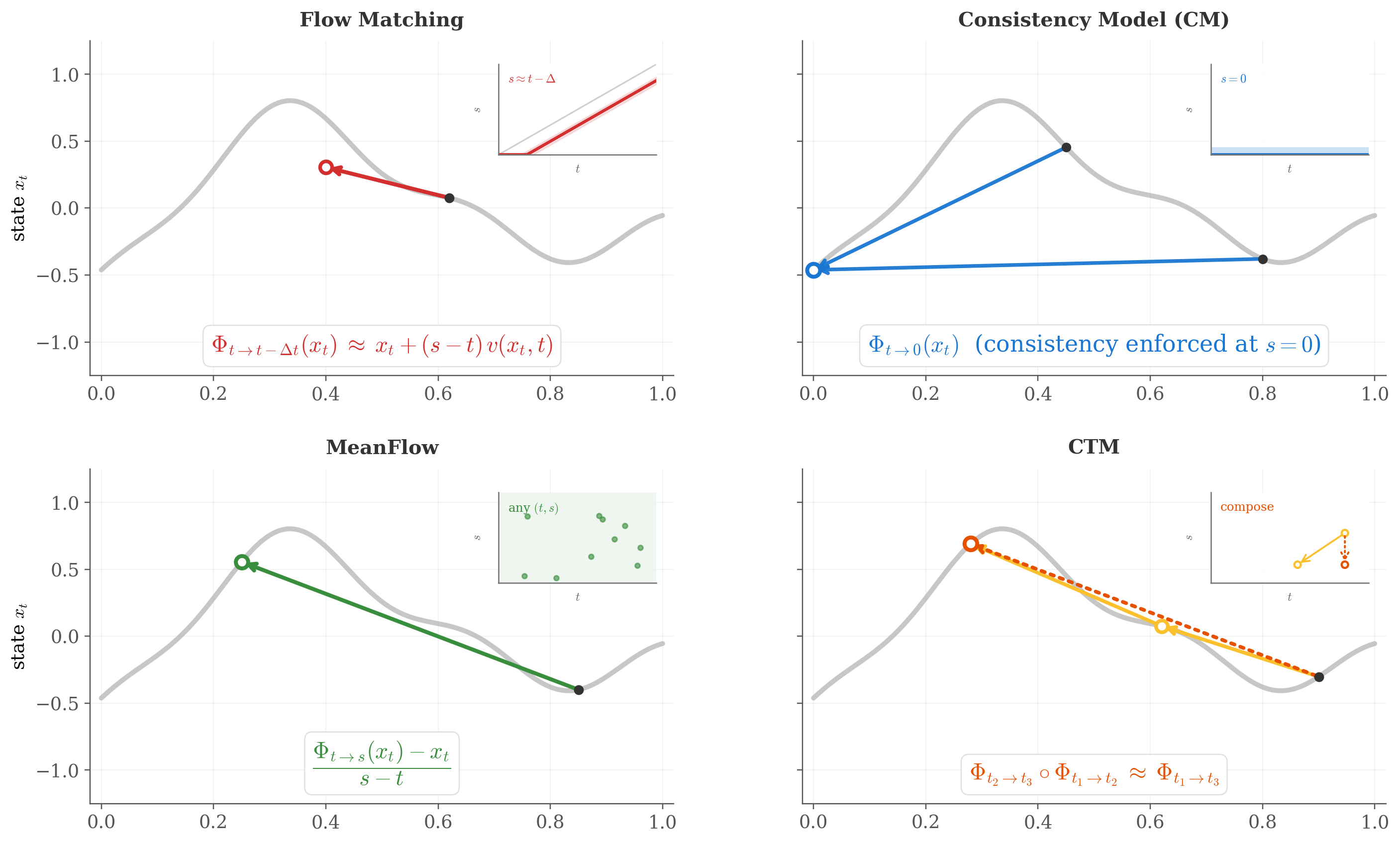
• Consistency Models (CM) as Boundary Operators: CMs restrict the target time to the data endpoint $s=0$ and learn only the boundary slice:

  \[f_\theta^{\text{CM}}(x_t, t) \equiv f_\theta(x_t, t, 0).\]

  Limitation: because the model never represents $s>0$ explicitly, arbitrary stop-and-go schedules (or back-and-forth edits) often require extra heuristics (e.g., go to $x_0$ then re-noise), which can accumulate error across hops.

• Flow Matching (FM) as the Infinitesimal Limit: Flow Matching learns the local velocity field $v_\phi(x,t)$. In flow-map language, this corresponds to learning the first-order infinitesimal behavior of the operator:

  \[v_\phi(x,t) = \lim_{s\to t} \frac{f_\theta(x, t, s) - x}{s-t}.\]

  Limitation: to realize a finite jump $t\to s$, we still need numerical integration (many NFEs), unless further distilled.

• MeanFlow as a Linearized Operator: MeanFlow ⁶ parameterizes a restricted family of operators using an average velocity $u_\theta$:

  \[f_\theta(x, t, s) = x + (s-t)u_\theta(x, t, s).\]

  where the ideal target is the time-average

  \[u_{\theta}(x_t,t,s) \approx \frac{1}{s-t}\,\int_{t}^{s} v_\theta(x_\tau,\tau)\,d\tau.\]

• Consistency Trajectory Models (CTM) are Discrete Compositions: CTM ⁷ enforces the composition property on a discrete grid of time steps, acting as a discretized surrogate of the full flow map algebra:

  \[f_\theta(f_\theta(x, t_2, t_1), t_1, t_0) \approx f_\theta(x, t_2, t_0).\]

Under the operator-centric view, methods such as MeanFlow and Consistency Trajectory Models (CTM) can be interpreted as concrete instantiations of flow-map learning, differing mainly in parameterization and which parts of the two-time operator are explicitly represented and constrained.

2.3 Why Operators? Speed, Control, and Composability

Lifting the abstraction from trajectories to operators buys us three practical advantages:

1. Amortization of Integration (Speed): Once $f_\theta$ is trained, a finite jump $t\to s$ is a single network evaluation. Unlike boundary-only maps, the operator can directly target any intermediate $s$, rather than always “touching” $s=0$.

2. Decoupling Physics from Discretization (Control): Trajectory-based samplers entangle the ODE dynamics with the solver’s step size. With a flow map, the “desired jump” $(t, s)$ is an explicit input. This makes the model robust to changing step counts and enables non-uniform schedules tailored to specific editing tasks.

3. Algebraic consistency (Composability).
   Many real pipelines require chaining time jumps (e.g., iterative editing, refine-and-correct loops). If $f_\theta$ respects semigroup structure, then “direct” and “composed” jumps agree:

   \[\Phi_{t\to s}\approx \Phi_{u\to s}\circ\Phi_{t\to u},\]

   which directly suppresses drift accumulation. This gives us not only better behavior in composed pipelines, but also a concrete diagnostic: semigroup violation becomes a measurable unit test for learned generative operators.

3. Training Two-Time Operators via Eulerian and Lagrangian Distillation

In Chapter 2, we elevated generative modeling from integrating infinitesimal dynamics to learning finite-time operators. We now turn to the central practical question: how can we train a neural operator $$f_\theta(x_t, t, s) \approx \Phi_{t\to s}(x_t)$$ without placing an expensive ODE solver inside the training loop?

Assume we have a teacher dynamics (e.g., probability-flow ODE or rectified-flow ODE) governed by a velocity field

A naive approach would sample many $(t,s)$ pairs and numerically integrate the teacher from $t$ to $s$ to obtain supervision. This is prohibitively costly. Instead, we exploit two identities of flow maps:

• How the map changes when we move the target time $s$ (Lagrangian view),
• How the map changes when we move the start time $t$ (Eulerian view).

Both lead to one-step distillation losses that require only a small teacher step / teacher velocity evaluation.

3.1 The Lagrangian View: Moving the End Point

Fix a starting state $x_t$ at time $t$, and view $\Phi_{t\to s}(x_t)$ as a function of the endpoint $s$. Following the same particle along the trajectory yields the standard identity (flow-map derivative in the target time):

Interpretation. As we move the endpoint $s$, the output moves according to the teacher velocity evaluated at the current location on the trajectory. This suggests a natural “predict-then-correct” distillation rule.

Lagrangian Map Distillation (LMD). Choose a small fraction $\varepsilon\in(0,1)$ and define an intermediate endpoint $$s' = s + \varepsilon (t-s), \qquad \text{so that } s < s' < t.$$ Then a first-order (backward-in-time) Euler correction from $s'$ to $s$ gives:

We implement this without integrating the teacher trajectory: we let a target/EMA network $f_{\theta^-}$ propose a state at time $s'$, and use the teacher velocity to correct it by one step. The LMD objective becomes:

Why this helps. LMD directly ties the predicted endpoint to the teacher dynamics: the student is trained to land on a state that is consistent with the teacher’s velocity at that future point. Empirically, this stabilizes “where you end up” for arbitrary $(t,s)$ jumps and reduces endpoint bias that often appears when a model is trained only to hit a single boundary (e.g., $s=0$).

3.2 The Eulerian View: Moving the Start Point

Now fix the destination time $s$ and study how the operator changes when we perturb the start time $t$. This is an Eulerian viewpoint: instead of following a particle, we ask how the map itself must transform so that the final destination at time $s$ remains invariant.

From the semigroup law $\Phi_{t\to s} = \Phi_{t'\to s}\circ \Phi_{t\to t'}$ and a first-order expansion, one obtains the transport (backward) equation for ODE flow maps:

Equivalent “pre-transport” intuition. If we move the start time from $t$ to a slightly later (closer-to-$s$) time $t'$, we should first push the input $x_t$ along the teacher flow from $t$ to $t'$, and then apply the operator from $t'$ to $s$:

Eulerian Map Distillation (EMD). Pick the same $\varepsilon\in(0,1)$ and define $$t' = t + \varepsilon(s-t), \qquad \text{so that } s < t' < t.$$ We compute a single teacher Euler step to obtain $x_{t'}$ and enforce consistency under this transport:

Connection to consistency-style training. When $s$ is fixed to the boundary (e.g., $s=0$), this becomes the familiar “start-time invariance” constraint behind consistency-type objectives—here generalized to arbitrary destinations $s$.

3.3 Synthesis: A Unified Objective

LMD and EMD provide complementary supervision signals:

• Lagrangian (LMD) constrains endpoint correctness: the jump must land on a state that is locally consistent with the teacher velocity at the predicted location.
• Eulerian (EMD) constrains start-time consistency: shifting the start time and transporting the input accordingly should not change the final prediction.

A practical training objective is a weighted combination:

What this buys us. Unlike endpoint-only shortcuts, the combined objective learns a two-time primitive: it can jump to arbitrary $s$ (control), remains stable under varying step schedules (robustness), and is structurally aligned with semigroup composition (composability). This sets up the experimental questions in the next chapter: are learned jumps indeed less sensitive to NFE, and do they exhibit smaller drift under multi-hop composition?

4. Experiments: Step Robustness and Compositional Drift

In Chapters 2–3, we argued for a shift from trajectory integration (solving an SDE/ODE step-by-step) to operator learning (predicting a finite-time jump $\Phi_{t\to s}$ directly). This viewpoint yields two concrete, testable expectations:

1. Robustness to discretization (NFE): if inference is implemented by learned finite jumps, output quality should be less sensitive to the number of function evaluations (NFE), compared to solvers that rely on small-step approximations.
2. Algebraic consistency (semigroup behavior): a genuine two-time operator should approximately satisfy \(\Phi_{t\to s}\;\approx\;\Phi_{u\to s}\circ\Phi_{t\to u},\) so that direct and multi-hop composed jumps agree up to small error, and the discrepancy grows slowly with hop count.

We validate these points using two experiments under a shared inpainting setup:

• Exp-I (Sec. 4.3): compare integration-based samplers (SDE/ODE) versus jump-distilled samplers under different NFE budgets. This answers why jumps remain usable at very low steps.
• Exp-II (Sec. 4.4): compare direct \(t\!\to\!s\) versus $k$-hop composed jumps, and quantify the resulting composition drift. This operationalizes the semigroup diagnostic.

4.1 Shared experimental setup (common to both experiments)

Task: image inpainting. Given an image \(x\in\mathbb{R}^{H\times W}\) and a binary mask \(m\in\{0,1\}^{H\times W}\), the goal is to fill the masked region $\Omega$ (where \(\Omega=\{(i,j) \mid m_{ij}=1\}\)) in a way consistent with the context and text prompt. This is a good stress test for step robustness because failures often show up as geometry glitches or texture incoherence when NFEs are too small.

Backbone & pipeline. We use the same Stable Diffusion v1.5 inpainting backbone instantiated via AutoPipelineForInpainting, and vary only the scheduler / distilled head (LoRA) depending on the method.

Methods. We compare four inference paradigms built on the same backbone (same prompt encoder / VAE / UNet weights unless stated otherwise):

• SDE-like sampler: Euler ancestral discretization (EulerAncestralDiscreteScheduler).
• ODE-like sampler (probability-flow style): deterministic DDIM (DDIMScheduler, \(\eta=0\)).
• Endpoint-jump distillation (CM-like, proxy): LCMScheduler ⁸ with an LCM LoRA fused into the pipeline.
• Two-time jump distillation (Flow-like, proxy): TCDScheduler ⁹ with a TCD LoRA fused into the pipeline (used as a practical approximation to “two-time operator distillation”).

Fairness controls (Exp-I & Exp-II). To isolate step/schedule effects rather than prompt/guidance variance, we enforce:

• Same inpainting input (image + mask) and same prompt/negative prompt.
• Same step budgets (Exp-I uses ({2,4,8,16,30}), and Exp-II uses ({2,4,6,8})).
• Same random seed and the same guidance scale across all methods.

Extra controls for composition drift (Exp-II). Because composition drift is subtle, we add two controls specifically for Exp-II:

• Fixed noise for the endpoint re-noise step in the CM-proxy, so drift reflects structural inconsistency rather than stochastic variance.
• Unmasked-region locking: we explicitly lock the unmasked context region to a shared reference latent trajectory at every intermediate time, ensuring the metric measures drift only inside the edited region.

4.2 A note on “proxies”

A key practical detail is that we do not train a full flow-map network \(f_\theta(x_t,t,s)\) from scratch in this blog post. Instead, we use public distilled LoRAs ¹⁰ as stand-ins for two different structural paradigms:

• LCM-LoRA as an endpoint-jump proxy (CM-like): it behaves like a boundary map \(B_t(x_t)\approx x_0\), and any \(t\to s\) jump is synthesized via “denoise to $x_0$, then re-noise to $s$”.

• TCD-LoRA as a two-time-jump proxy (Flow-like): we treat the model as supporting a DDIM-coupled jump \(a\to b\) that depends on the target time through \((\alpha_b,\sigma_b)\), rather than always anchoring at \(t=0\).

Concretely, in Exp-II we instantiate two “operators”:

• Flow-proxy jump (DDIM-coupled):

  \[\Phi^{\text{flow}}_{a\to b}(x_a) = \frac{\alpha_b}{\alpha_a} x_a + \Bigl(\sigma_b-\frac{\alpha_b}{\alpha_a}\sigma_a\Bigr)\,\varepsilon_\theta(x_a,a),\]

  where \(\varepsilon_\theta\) comes from the TCD-distilled predictor and \((\alpha_t,\sigma_t)\) are from a reference DDIM schedule.

• CM-proxy jump (endpoint-anchored):

  \[\Phi^{\text{CM}}_{a\to b}(x_a) = \alpha_b\,B_a(x_a) + \sigma_b\,\epsilon_0,\]

  where \(B_a(x_a)\) is a learned endpoint map: \(x_a \to x_0\), comes with a fixed \(\epsilon_0\) shared across all compositions.

Why this is still meaningful. Our goal is not to claim “we trained the definitive flow map.” The goal is to empirically test a structural hypothesis from Chapters 2–3: multi-hop pipelines should be more stable when the underlying primitive is a genuine two-time operator (semigroup-consistent), and less stable when every hop must “return to \(x_0\)” as an anchor.

Even with proxies, Exp-II directly measures the semigroup violation diagnostic (direct vs composed). As long as the two proxies reflect the two paradigms (endpoint-anchored vs time-to-time jump), the diagnostic remains aligned with the theory.

Limitation (explicit): the absolute numerical values of drift depend on the particular checkpoints; a true \(f_\theta(x_t,t,s)\) trained with explicit composition constraints could reduce drift further. We view the proxy study as an evidence-of-principle validation.

4.3 Exp-I: Inpainting under different NFEs (Robustness to Discretization)

We first test whether jump-based inference indeed reduces step sensitivity. Using the common setup in Sec. 4.1, we run each method with step counts ({2,4,8,16,30}) and visualize the inpainted outputs, as shown in Figure 2.

Figure 2. Inpainting results vs NFE. Integration-based samplers (SDE/ODE) are sensitive to step count; jump-distilled samplers (LCM/TCD) are stable at very small NFEs.

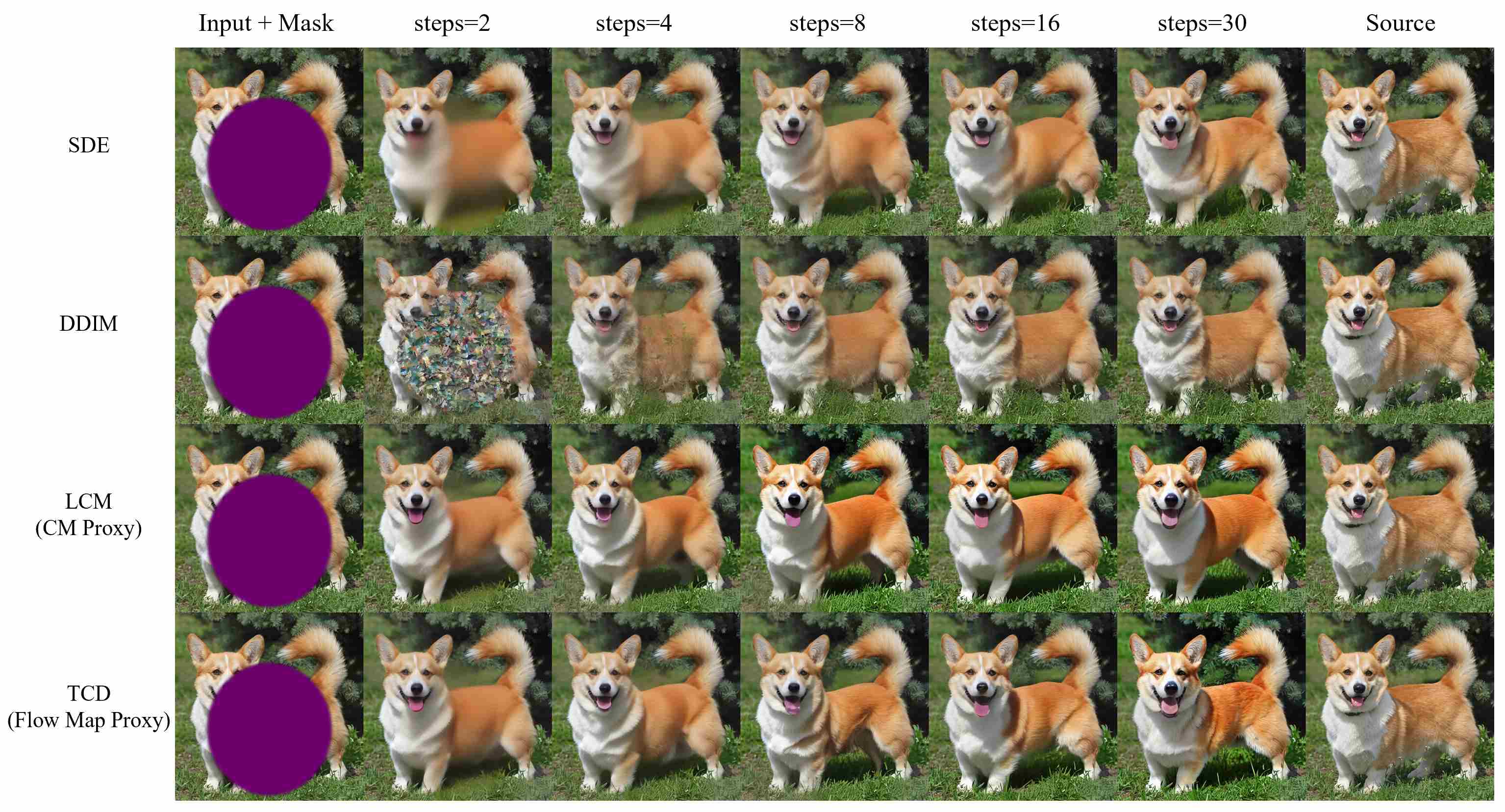
Observation. The qualitative trend is consistent:

• SDE/ODE (integration) are notably worse at very low NFEs and improve as NFEs increase, as expected from discretization/integration error accumulation.

• LCM/TCD (jump-distilled) already produce plausible inpaintings at 2 steps and change less across the step range.

Interpretation. This experiment supports the “trajectory vs operator” narrative: once inference is amortized into learned jumps, the output becomes less tied to the solver resolution (step count). Importantly, Exp-I is not meant to separate CM vs FlowMap; at this level both are “jump” methods, so the main takeaway is jump distillation vs integration.

4.4 Exp-II: Direct vs composed jumps (composition drift diagnostic)

Exp-I shows that jump distillation helps at low NFEs. Exp-II asks a stricter question tied to flow-map algebra: If we want to jump from $t$ to $s$, does it matter whether we do it directly, or via multiple intermediate hops?

Protocol Setup: direct vs $k$-hop composition

For each trial we sample a start time $t$, an end time \(s\approx 0\), and \(k-1\) intermediate times

We compare:

• Direct:

  \[x_s^{\text{dir}} = \Phi_{t\to s}(x_t)\]

• Composed:

  \[x_s^{\text{comp}} = \Phi_{u_{k-1}\to s}\circ\cdots\circ\Phi_{t\to u_1}(x_t)\]

Ideally, for a valid flow map, Direct $\approx$ Composed. We define the Compositional Drift as the Mean Squared Error (MSE) between these two outputs in the latent space.

Quantitative Result: Error Accumulation

Figure 3. Composition drift $\Delta_k$ (masked latent MSE, log-scale) vs hop count. Flow-proxy (TCD) shows much smaller drift and slower growth than CM-proxy (LCM).

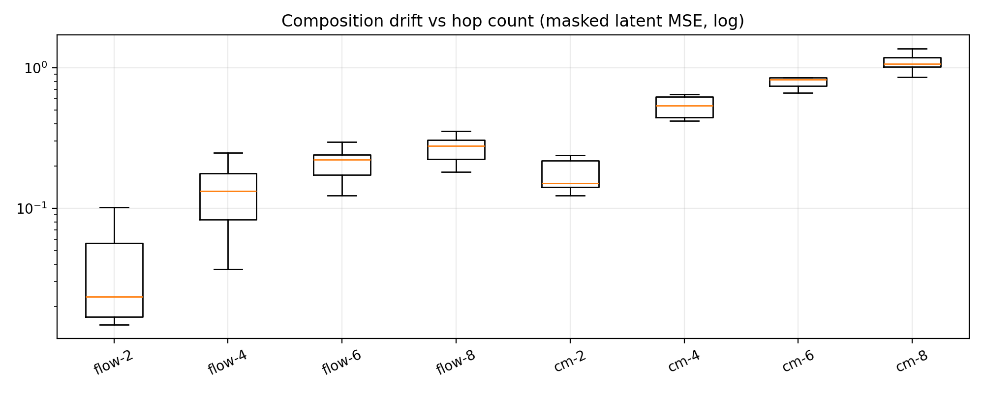
Figure 3 reveals a stark difference in algebraic properties:

• Flow Map (Left): The drift is minimal ($10^{-2}$ range) and grows slowly with hops. This indicates the model has learned a “straight” transport path where $\Phi_{t \to s}$ acts as a true semi-group.
• CM (Right): The drift is an order of magnitude larger ($10^{-1} \to 10^0$) and grows faster than Flow Map. Every time the CM “touches the boundary” ($x_0$) and comes back, it introduces prediction error that compounds rapidly.

Qualitative Result: Semantic Drift

To make the effect tangible, we also decode “direct vs composed” and visualize \(\|\Delta\|\) in image space (masked region only). Under ideal semigroup consistency (direct \(\approx\) composed), the residual map \(\|\Delta\|\) should be negligible (nearly black).

Figure 4. Qualitative examples of direct vs 8-hop composed jumps. Flow-proxy remains nearly invariant; CM-proxy shows visible structural drift, highlighted by brighter $\mid \Delta \mid$ maps.

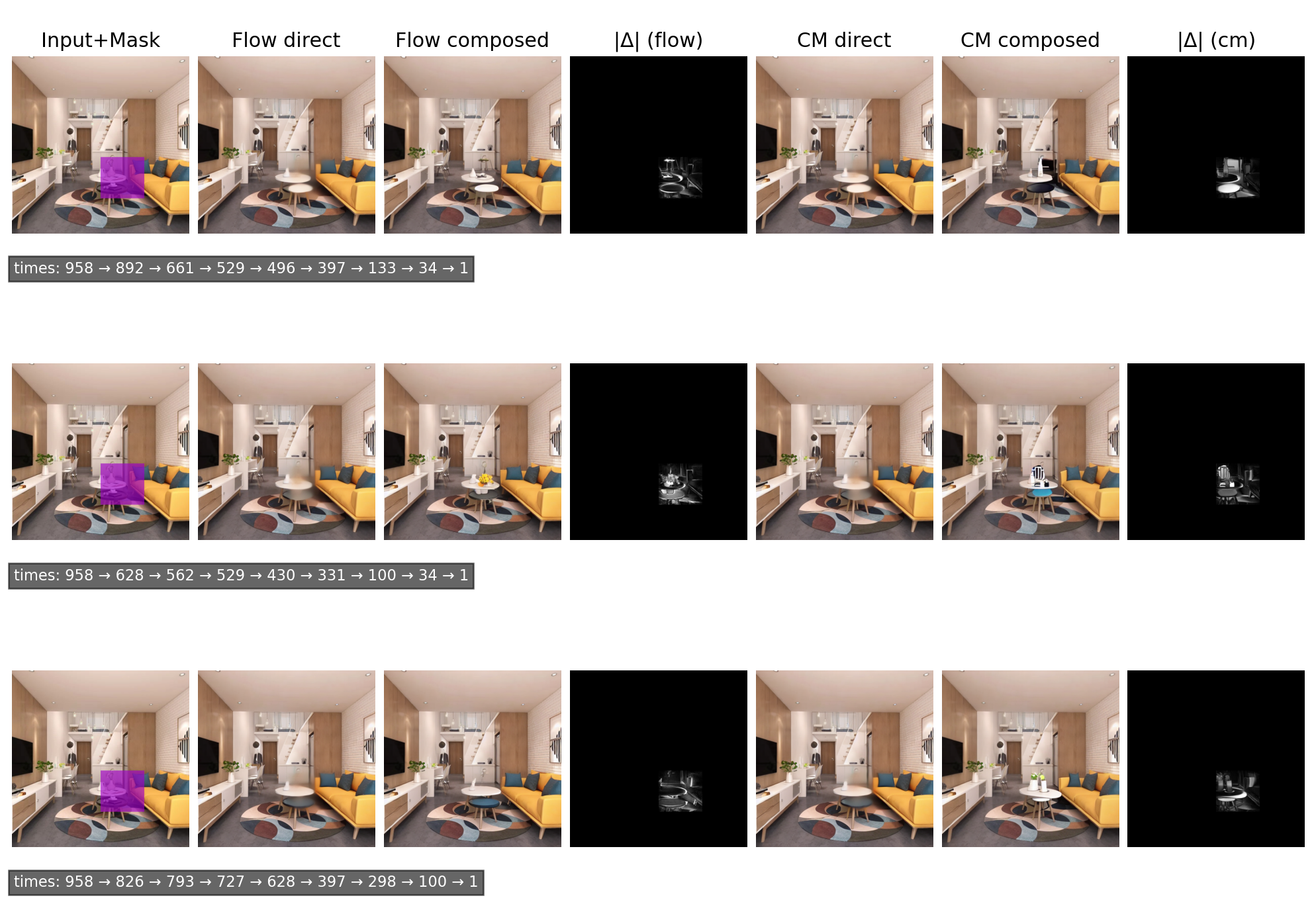
• CM Failure: The “CM Composed” image shows the object on the stool mutating into a black-and-white artifact. The $|\Delta|$ map is bright, indicating severe pixel-level deviation.

• Flow Success: The “Flow Composed” image is visually closer to the “Direct” one. The $|\Delta|$ map is nearly black.

Interpretation. This experiment operationalizes semigroup consistency: the flow-proxy behaves closer to a path-independent two-time operator, while the endpoint-anchored CM-proxy accumulates drift because each hop reprojects to an estimated \(x_0\) and then re-noises—small endpoint errors become amplified across hops.

5. Conclusion

This post advocated a simple shift in abstraction: from integrating trajectories to learning operators. Instead of treating sampling as the repeated numerical solution of an ODE/SDE, we view generation as composing finite-time maps. The flow map family \(\{\Phi_{t\to s}\}\) is the minimal object that retains control (arbitrary start/stop times) while enabling speed (amortized jumps), and its algebraic structure—identity and the semigroup law—acts as the “physics” that distinguishes a genuine two-time operator from a boundary-only shortcut.

We then showed how this operator view organizes a large body of recent work:

• Consistency Models emerge as boundary operators \(f_\theta(x_t,t,0)\), fast but structurally rigid.
• Flow Matching is the infinitesimal limit of a flow map, flexible but expensive at inference.
• MeanFlow and CTM can be interpreted as intermediate points that impose linearization or discrete composition constraints.

On the training side, we derived two complementary distillation perspectives:

• The Lagrangian view (LMD) supervises how the endpoint moves with the target time $s$, anchoring the operator to the teacher’s dynamics.
• The Eulerian view (EMD) supervises how the operator evolves with the start time $t$, enforcing invariance under transport and connecting naturally to consistency-style objectives.

Together, they suggest that “learning \(\Phi_{t\to s}\)” is not a single recipe but a design space: which derivatives you match (and how strongly you enforce composition) determines how well the learned operator behaves under chaining and editing.

Finally, we proposed two concrete, falsifiable hypotheses for operator learning and tested them under a shared inpainting setup:

1. Robustness to discretization: jump-based inference should be less sensitive to the step budget than integration-based sampling.

2. Algebraic consistency: if an operator is semigroup-consistent, direct and composed jumps should agree, and the discrepancy should grow slowly with hop count.

Even with practical proxies (LCM as endpoint-anchored, TCD as DDIM-coupled two-time jump), the experiments support the central narrative: operator-like jumps are step-robust, and two-time jumps exhibit substantially lower compositional drift than endpoint-anchored hops. This points to a useful takeaway beyond any specific method: “semigroup violation” can serve as a unit test for generative operators, especially in pipelines that repeatedly jump across time (editing, multi-stage refinement, or back-and-forth schedules).

Limitations and Outlook

Our study deliberately prioritized structure over full-scale training: we did not train a complete \(f_\theta(x_t,t,s)\) with explicit semigroup regularization. The next step is therefore clear: train true flow maps with (i) broad coverage over $(t,s)$, (ii) explicit composition constraints, and (iii) evaluation on tasks where chaining is unavoidable (e.g., iterative editing loops, guided refinement schedules, and long-horizon compositions). If successful, operator learning could offer a principled route to fast generation that remains composable, controllable, and stable under changing schedules—precisely where many endpoint-anchored distillations tend to break.

6. References