
Discrete Visual Tokenizers for Multimodal LLMs: Bridging Vision and Language
📅 Published: | 🔄 Updated:
📘 TABLE OF CONTENTS
- 1. Foundations of Visual Tokenization
- 2. Quantization in Visual Tokenizers: Two Orthogonal Axes
- 3. Explicit codebooks: Vector Quantization Families
- 4. Codebook Update Dynamics
- 5. Codebook Initialization Design
- 6. Objective function Design for Higher Utilization and Diversity
- 7. Codebook Architecture Design
- 8. Implicit / codebook-free quantizers
- 9. References
Representation learning fundamentally concerns transforming raw signals into compact latent representations. These representations take two forms: continuous representations as real-valued vectors, and discrete representations as symbolic tokens from finite vocabularies. While continuous methods have long dominated visual representation learning, discrete representations offer distinctive advantages—combinatorial expressiveness, compatibility with symbolic reasoning, and natural integration with large language models—that prove essential for multimodal AI systems.
1. Foundations of Visual Tokenization
Visual tokenization pipelines typically follow the same skeleton:
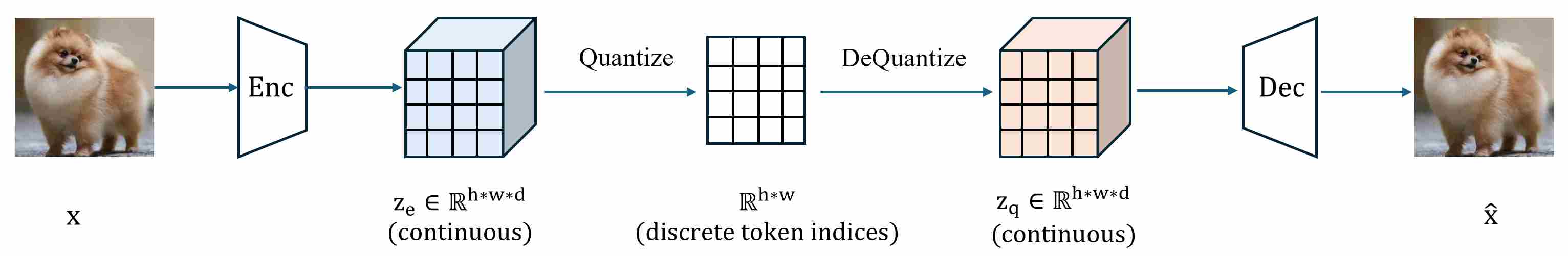
The quantizer is the “discrete interface” that makes images/videos compatible with token-based models (Transformers, LLM-style decoders, entropy coders, etc.). A quantizer is a computational module that transforms continuous visual signals (Encoder output $z_e$) into discrete symbolic representations. Formally, given an input \(\mathbf{z_e}\in\mathbb{R}^{h\times w\times d}\), a visual tokenizer is a learned (or partially fixed) mapping
\[\mathcal{T}: \mathbf{z_e}\in\mathbb{R}^{h\times w\times d}\ \mapsto\ \mathcal{V}^N\]where \(\mathcal{V}=\{1,2,\dots, K\}\) denotes a finite vocabulary of size $K$, and $N$ represents the number of output tokens. Two major families dominate:
Codebook-based (explicit) quantization: learn a set of embeddings (a dictionary) and map $z_e$ to its nearest entry. Representative algorithms include VQ-VAE 1, VQ-VAE-2 2, VQ-GAN 3, ViT-VQGAN 4.
Codebook-free (implicit) quantization: map $z_e$ to discrete codes using fixed rules or structured parameter-free operators. Representative algorithms include FSQ 5, LFQ 6, BSQ 7.
Both families must address the same core training friction: hard discretization is not differentiable, so most systems rely on surrogate gradients (often STE) or continuous relaxations in some form. The key differences are where the difficulty concentrates: codebook-based methods struggle with learning and maintaining the dictionary; codebook-free methods focus on structuring the discrete space so it is stable, scalable, and hardware-friendly.
1.1 The core benefits
Compared with continuous representation, discrete tokenizers are not better universally. Instead, they are a design choice that becomes attractive when your downstream model or objective aligns with discrete structure.
Benefit 1 — Compatibility with Large Language Models
LLMs are optimized for sequences of discrete token IDs. Discrete vision tokens let you reuse (almost) the same learning machinery—autoregressive modeling, masked token prediction, next-token loss, etc. — without inventing new continuous likelihood objectives.
Benefit 2 — Compression that is countable (sequence length as a first-class resource)
For token models, the dominant cost is often tied to sequence length $N$ (attention, KV cache, decoding steps). Discrete tokenizers turn “how big is the image” into “how many tokens do we spend.” This makes the compute–quality trade-off explicit and controllable.
Benefit 3 — Strong priors become easier to express and evaluate
A discrete latent space supports powerful priors $p(\mathbf{z})$ (AR, masked generative models). VQ-VAE emphasizes learning a discrete latent structure and then training a powerful prior over those discrete variables.
1.2 The Evolution of Discrete Tokenization
The trajectory of discrete tokenization has not been linear, it is a history defined by shifting paradigms and evolving objectives.
Stage 1 — Reconstruction-Oriented Discrete Representation
The genesis of visual discrete tokenization can be traced to the Vector Quantized Variational Autoencoder (VQ-VAE), which introduced learnable discrete codebooks as an intermediate representation between encoder and decoder networks. By replacing continuous VAEs’ KL-regularized bottlenecks with a quantized latent interface, thereby reducing the tendency of powerful decoders to ignore the latent signal (a key failure mode behind posterior collapse).
Objective: The overarching goal was service-oriented, i,e,. providing a high-fidelity discrete interface for generative models
Core Focus: The central challenge lay in the design of the discrete codebook. Early approaches, such as VQ-VAE, introduced vector quantization to compress visual information but struggled with codebook collapse and low utilization. Subsequent advancements, exemplified by VQ-GAN and VQ-VAE-2, incorporated perceptual and adversarial losses (e.g., LPIPS, discriminator loss) to dramatically enhance reconstruction quality. Techniques like Exponential Moving Average (EMA) updates and restart heuristics were developed to stabilize training.
Representative Works of Stage 1 can be summarized as follows
| Method | Modality | Codebook | Token Layout | Vocab Size | Key Contribution |
|---|---|---|---|---|---|
| VQ-VAE 1 | Image | Learned | 2D | 512 | Discrete latent via vector quantization |
| VQ-VAE-2 2 | Image | Learned | 2D (hierarchical) | 512 per level | Multi-scale hierarchical codebooks |
| DALL-E dVAE 8 | Image | Learned | 2D | 8192 | Gumbel-softmax relaxation, large vocab |
| VQ-GAN 3 | Image | Learned | 2D | 1024–16384 | Adversarial + perceptual losses |
| RQ-VAE 9 | Image | Learned (residual) | 2D × D | 16384 × depth | Residual quantization for finer granularity |
| ViT-VQGAN 4 | Image | Learned | 2D | 8192 | ViT-based encoder-decoder architecture |
Stage 2 — Representation Learning via Discrete Targets
The second phase witnessed a paradigm shift wherein discrete visual tokens transitioned from serving as generative bottlenecks to functioning as self-supervised learning targets. This evolution was catalyzed by two concurrent developments: the remarkable success of Vision Transformers (ViT) in establishing Transformers as viable vision backbones, and the desire to transfer the masked language modeling paradigm from NLP to the visual domain.
BEiT pioneered this approach by proposing Bidirectional Encoder representation from Image Transformers, which leverages discrete visual tokens from a pretrained VQ-VAE as prediction targets for masked image patches. Unlike pixel-level regression objectives, discrete tokens provide a more semantically meaningful supervision signal while naturally handling the inherent ambiguity of visual reconstruction. The discrete vocabulary imposes an information bottleneck that encourages the encoder to learn high-level semantic features rather than low-level textural details.
Subsequent works further enhanced this framework by improving the semantic quality of target tokens. BEiTv2 introduced a vector-quantized knowledge distillation mechanism that aligns discrete tokens with semantically rich features from pretrained models. PeCo proposed perceptual codebooks optimized with perceptual losses to better capture human-relevant visual features. These developments revealed a critical insight: the quality of discrete tokenization fundamentally determines the ceiling of downstream task performance, as the tokenizer defines the granularity and semantic level of the learning objective.
It is worth noting that this phase coincided with, rather than being displaced by, the rise of diffusion models. While diffusion models gradually dominated generative tasks through superior sample quality, discrete tokenization found renewed purpose as a vehicle for discriminative pretraining, demonstrating the versatility of the discrete representation paradigm.
Representative Works of Stage 2 can be summarized as follows
| Method | Modality | Codebook | Token Layout | Vocab Size | Key Contribution |
|---|---|---|---|---|---|
| iGPT 10 | Image | Color palette | 1D (raster) | 512 colors | Autoregressive pretraining on pixels |
| BEiT 11 | Image | Pretrained dVAE | 2D | 8192 | Masked image modeling with discrete targets |
| PeCo 12 | Image | Perceptual | 2D | 8192 | Perceptual codebook for better semantics |
| BEiTv2 13 | Image | VQ-KD | 2D | 8192 | Knowledge distillation for semantic tokens |
| BEiT-3 14 | Image+Text | Shared | 2D + 1D | 64010 | Multimodal masked modeling |
| MAGE 15 | Image | VQ-GAN | 2D | 1024 | Unified generation and representation |
| MaskGIT 16 | Image | VQ-GAN | 2D | 1024 | Non-autoregressive parallel decoding |
Stage 3 — Native Multimodal large language models, unified understanding and generation
The emergence of Large Language Models (LLMs) and their extraordinary capabilities in reasoning and generation has fundamentally reshaped the landscape of visual tokenization. The third and current phase is characterized by the pursuit of native multimodal architectures wherein visual and linguistic tokens coexist within a unified vocabulary and are processed by a single autoregressive transformer. This paradigm enables true end-to-end training across modalities and facilitates the seamless unification of understanding and generation tasks.
This phase introduces a distinct set of technical challenges. First, the semantic-perceptual trade-off becomes paramount: tokenizers optimized purely for reconstruction (e.g., VQ-GAN) excel at preserving low-level visual fidelity but may discard semantic information critical for understanding tasks. Conversely, semantically-aligned tokenizers (e.g., those distilled from CLIP) capture high-level concepts but struggle with fine-grained reconstruction. Recent works such as SEED and Emu have proposed hybrid objectives that jointly optimize for both semantic alignment and visual reconstruction, often through multi-stage training or auxiliary loss functions.
Second, compression efficiency and bitrate optimization have gained renewed attention. Native multimodal models must balance the competing demands of token budget (affecting sequence length and computational cost), reconstruction quality, and semantic preservation. This has motivated the development of novel quantization schemes. Finite Scalar Quantization (FSQ) discretizes each latent dimension to a predefined set of levels, eliminating the learned codebook entirely and thus circumventing codebook collapse by construction. Lookup-Free Quantization (LFQ) similarly eschews explicit codebook storage by deriving discrete indices through binary or multi-level quantization of latent dimensions. Residual Quantization (RQ) applies successive quantization stages to residual errors, enabling fine-grained reconstruction with variable-rate encoding.
Third, the extension to video tokenization introduces additional complexity through the temporal dimension. MAGVIT and its successor MAGVIT-2 pioneered spatiotemporal tokenization by extending 2D codebooks to 3D causal architectures, enabling both image and video processing within a unified framework. The recent Cosmos Tokenizer further advances this direction with state-of-the-art compression ratios while maintaining temporal coherence.
Finally, architectural innovations in generation paradigms have expanded beyond pure autoregressive modeling. MaskGIT demonstrated that parallel decoding through iterative mask refinement can achieve competitive quality with significantly reduced inference latency. More recent works such as MAR (Masked Autoregressive Models) and Transfusion explore hybrid approaches that combine the flexibility of autoregressive factorization with the efficiency of parallel sampling or the quality of diffusion-based refinement.
Representative Works (Image) of Stage 3 can be summarized as follows
| Method | Codebook Type | Token Layout | Vocab Size | Semantic Aligned | Key Contribution |
|---|---|---|---|---|---|
| SEED 17 | Learned + CLIP | 1D (causal) | 8192 | ✓ | Semantic tokenizer for MLLMs |
| SEED-2 18 | Learned + CLIP | 1D (causal) | 8192 | ✓ | Unified image-text generation |
| LaVIT 19 | Dynamic | 1D (variable) | 16384 | ✓ | Dynamic token allocation |
| Emu 20 | Learned (CLIP init) | 2D | 8192 | ✓ | Multimodal autoregressive |
| Emu3 21 | Learned | 2D | 32768 | Partial | Next-token prediction only |
| Chameleon 22 | Learned | 2D | 8192 | × | End-to-end native multimodal |
| Show-o 23 | MAGVIT-2 | 2D | 8192 | × | Unified AR + Diffusion |
| Janus 24 | Decoupled | 2D | 16384 | Decoupled | Separate understanding/generation paths |
| LlamaGen 25 | VQ-GAN | 2D | 16384 | × | Class-conditional AR generation |
| Open-MAGVIT2 26 | LFQ | 2D | 262144 | × | Lookup-free, large vocab |
| TiTok 27 | Learned | 1D | 4096 | × | Compact 1D image tokenization |
Stage 4 — Recent Trends (2024–): Scaling, Stability, and Evaluation
As codebooks scale to \(2^{18}\) tokens and beyond, training stability becomes a first-order problem. Recent work such as Index Backpropagation Quantization (IBQ) 28 proposes making the full codebook differentiable via straight-through gradients on the one-hot assignment, enabling stable large-vocabulary tokenizers with high utilization.
Meanwhile, the community has started to build tokenizer-specific benchmarks. Instead of only reporting rFID / rFVD, benchmarks like TokBench / VTBench explicitly evaluate fine-grained preservation of text and faces, which often bottleneck downstream generation quality.
2. Quantization in Visual Tokenizers: Two Orthogonal Axes
In Vector Quantization (VQ) based generative models, the tokenizer must bridge the continuous latent space of the encoder and the discrete nature of tokens. Visual tokenization pipelines typically follow the same skeleton:
\[x \xrightarrow{\text{Encoder}} z_e \xrightarrow{\text{Quantizer}} z_q \xrightarrow{\text{Decoder}} \hat{x},\]where the quantizer forms the discrete interface that turns continuous latents into discrete tokens for token-based priors (Transformers, LLM-style decoders, entropy coders, etc.). Designing a quantizer involves two fundamental architectural decisions:
- Axis A — Representation Strategy (The “Where”): Codebook-based (explicit) vs. Codebook-free (implicit).
The question is: How is the discrete vocabulary / code space defined and represented?- Explicit codebook: a learnable embedding table \(\{e_k\}_{k=1}^K\) that stores token vectors.
- Implicit / codebook-free: no learnable embedding table; tokens are defined by a (usually element-wise) quantization rule (often with small learnable projections).
- Axis B — Optimization Paradigm (The “How”): Hard vs. Soft assignment.
The question is: How do we optimize through the non-differentiable discretization?- Hard: deterministic assignment (\(\arg\min\)/round/sign) + surrogate gradients (STE), EMA updates, etc.
- Soft: continuous relaxation (soft assignment / Gumbel-Softmax), often annealed to hard at the end.
These axes are complementary: any method can be positioned as a combination of (A) and (B). For example, classic VQ-VAE is explicit + hard, Gumbel-Softmax tokenizers are explicit + soft during training, and many modern codebook-free quantizers (FSQ/LFQ/BSQ) are implicit + hard (with STE) (optionally adding a temporary soft relaxation for stability).
2.1 Dimension I: Representation Strategies
The first dimension defines the structure of the discrete space $\mathcal{C}$ (the codebook) and how continuous vectors $z_e$ map to it.
2.1.1 Explicit Codebook (Codebook-based)
This is the classic approach and widely used in VQ-VAE, VQ-GAN, and ViT-VQGAN.
Mechanism: The model maintains a learned embedding table
\[E = \{e_1, e_2, ..., e_K\} \in \mathbb{R}^{K \times D}.\]Quantization is a nearest-neighbor lookup:
\[k = \operatorname*{argmin}_{j} \|z_e - e_j\|_2, \quad z_q = e_k\]Pros:
- Semantic Prototypes: The codebook learns a “visual vocabulary” where embeddings capture recurring semantic or textural patterns.
- Standard Interface: Provides a clean interface for downstream transformers (e.g., GPT) to predict token indices $k$.
Cons & Challenges:
- Codebook Collapse: A common failure mode where only a small subset of codes is used, while others become “dead codes.”
- Maintenance Overhead: Requires complex tricks to stabilize, such as EMA (Exponential Moving Average) updates, Codebook Reseeding (reviving dead codes), and Commitment Loss to bind the encoder to the embedding space.
2.1.2 Implicit Codebook (Codebook-Free)
Emerging methods like FSQ, LFQ, and BSQ remove the learned embedding table entirely. Instead, the “vocabulary” is defined implicitly by the quantization rule itself (e.g., a product space of scalar levels or binary bits).
Mechanism: Instead of a lookup, the latent $z_e$ is projected and discretized element-wise.
- FSQ (Finite Scalar Quantization): Projects $z_e$ to a low dimension, bounds it (e.g., via $\tanh$), and rounds it to a fixed set of integer levels \(\{1, \dots, L\}\). The codebook is the Cartesian product of these levels.
- LFQ (Lookup-Free Quantization): Binarizes the latent vector: \(z_q = \text{sign}(z_e) \in \{-1, 1\}^D\). The resulting binary string forms the token index.
- BSQ (Binary Spherical Quantization): Projects vectors onto a unit hypersphere before binarization, leveraging spherical geometry for better packing.
Pros:
- Stability: “Dead codes” are structurally impossible because there is no stored table to update.
- Infinite Scalability: The vocabulary size scales exponentially with dimension (e.g., $2^{12}$ bits vs. a fixed size $K$).
- Efficiency: operations are element-wise, avoiding expensive pairwise distance calculations.
Cons:
- Less Adaptivity: The lattice is fixed (hypercube or sphere corners) and cannot “move” to fit the data distribution like learned centroids.
2.2 Dimension II: Optimization Paradigms
Regardless of whether the codebook is Explicit or Implicit, the operation $z \to q(z)$ (argmin, round, or sign) is non-differentiable. To train the encoder via backpropagation, we must bridge this gap using either Hard or Soft strategies.
2.2.1 Hard Quantization
Hard quantization follows a “winner-takes-all” rule: each continuous latent \(z_e(x)\) is mapped to a single discrete choice. In the codebook-based setting, this is typically nearest-neighbor assignment:
\[z_q(x)=e_k,\quad k=\arg\min_{j\in{1,\dots,K}}\|z_e(x)-e_j\|_2^2.\]This produces true discrete tokens (indices $k$) and a clean interface for downstream token modeling.
However, the \(\arg\min\) is non-differentiable, so gradients cannot flow through the discrete selection. A standard workaround is the Straight-Through Estimator (STE): keep the hard assignment in the forward pass, but “copy” gradients in the backward pass:
\[\frac{\partial \mathcal{L}}{\partial z_e}=\frac{\partial \mathcal{L}}{\partial z_q}, \qquad z_q = z_e + (z_q - z_e).\text{detach}().\]Representative examples include VQ-VAE and VQ-GAN.
Note (connection to codebook-free): “Hard” does not imply “explicit codebook”. Many codebook-free quantizers also use hard discretization (e.g., round/sign), and still rely on STE-style surrogate gradients—only the discrete set is defined by a rule rather than a learned embedding table.
2.2.2 Soft Quantization: continuous relaxation of discrete assignment
Soft quantization replaces the hard, single-choice assignment with a differentiable mixture over all codes. In an explicit codebook setting:
\[z_q(x)=\sum_{j=1}^K p_j e_j,\qquad p=\mathrm{Softmax}(d/\tau),\]where $d$ is typically a similarity score (e.g., negative distances) and $\tau$ is a temperature controlling how “hard” or “soft” the distribution is. As \(\tau\to 0\), the distribution becomes close to one-hot (approaching hard assignment), while larger $\tau$ yields a smoother mixture. In practice, training often uses temperature annealing: start with higher $\tau$ for stable gradients and exploration, then gradually reduce $\tau$ to approach discrete behavior.
Soft quantization is differentiable “by construction”, but it introduces an important practical trade-off: if downstream usage requires discrete token IDs, one must eventually “harden” the assignment (e.g., argmax or sampling), which can create train–test mismatch if not handled carefully.
2.2.3 Gumbel-Softmax: stochastic soft quantization for categorical sampling
A widely used variant is Gumbel-Softmax, which injects Gumbel noise into logits before the softmax:
\[p=\mathrm{Softmax}\big((d+g)/\tau\big),\]where
\[g = -\log (-\log u)\qquad \text{and}\, u \sim {\mathrm Uniform}(0,1)\]This allows for sampling from a categorical distribution while maintaining differentiability via the reparameterization trick. This is especially useful when you want training-time behavior to more closely resemble discrete sampling rather than a deterministic mixture.
2.3 A Unifying View and Practical Takeaways
The landscape of discrete representation learning can be summarized by the intersection of these two dimensions:
| Hard Quantization (STE) Training = Inference | Soft Quantization (Relaxation) Differentiable approx. | |
|---|---|---|
| Explicit Codebook (Learned Dictionary) | The Standard (VQ-VAE/GAN) Requires codebook management (EMA/Restart) but offers high semantic fidelity. | Soft-VQ / Gumbel-VQ Used to stabilize early training or for specific probabilistic models. |
| Implicit Codebook (Fixed Rules) | The New Wave (FSQ / LFQ) High throughput, no collapse, highly scalable. Relies heavily on STE. | Relaxed Binary Using $\tanh$ or $\text{sigmoid}$ to approximate binary codes (common in Binary Neural Networks). |
In modern foundation-model pipelines, a common and effective recipe is to mix both worlds: train with soft relaxations when stability matters, then harden to discrete token IDs when discrete modeling or deployment requires it.
Inference-time (tokenization): almost always Hard
No matter whether the “codebook” is explicit or implicit, inference needs a discrete token id sequence for AR/MLM generators—so the forward quantizer at inference is hard:
- Explicit codebook → hard nearest-neighbor / argmin (classic VQ-style).
- Implicit codebook → hard rounding/sign/binarization (lookup-free / non-parametric style), e.g. LFQ uses sign to get binary latents and then maps them to token indices.
- BSQ does binary quantization after projecting to a hypersphere, then uses the resulting discrete representation as tokens.
Takeaway: Inference is hard; “soft” rarely appears as the final emitted tokenization.
Training-time (learning the tokenizer): Hard-forward is the default; Soft is usually auxiliary
The dominant recipe: Hard forward + surrogate gradients (STE). Training wants to match inference behavior, so SOTA tokenizers usually keep the forward quantization hard and use a straight-through gradient (or close variants) to backpropagate:
- FSQ: explicitly says it uses STE to get gradients through rounding, and emphasizes the codebook is implicit.
- Many VQ-style systems likewise rely on STE-style backprop through hard assignment; FSQ even contrasts VQ vs FSQ in a table: VQ has a learned codebook + extra losses/tricks, while FSQ has no learned codebook parameters and still uses STE.
Where “Soft” shows up in SOTA mostly for entropy/bitrate/utilization modeling
Even when the token is hard, SOTA often introduces soft probabilities in the loss (not necessarily in the emitted token stream):
- MAGVIT-v2 (LFQ): replaces the codebook embedding dimension with an integer set (implicit/codebook-free), uses sign for hard binary latents, and adds an entropy penalty during training to encourage utilization.
- BSQ: highlights (i) an implicit codebook with exponentially growing effective vocabulary and no learned parameters, and (ii) a soft quantization probability that factorizes into independent Bernoullis—useful for efficient entropy coding / regularization.
Takeaway: Soft is most often “auxiliary soft”—used to compute/regularize rate, entropy, or usage—while the main quantized path stays hard.
3. Explicit codebooks: Vector Quantization Families
The VQ was initially proposed to enhance the generation quality of VAE 29,30. A standard variational autoencoder (VAE) consists of an encoder and a decoder.
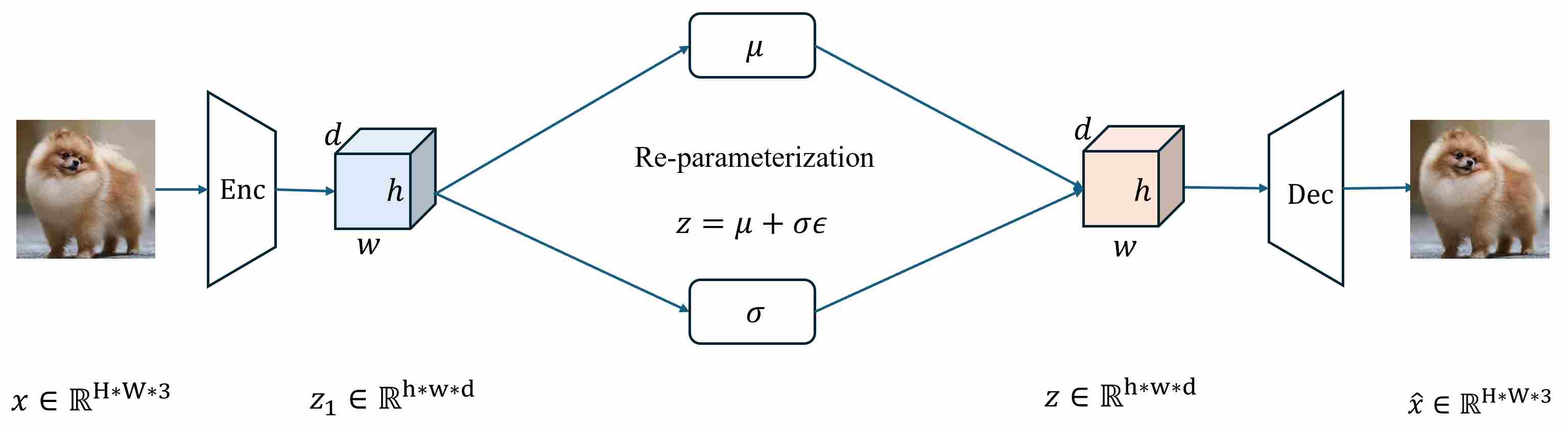
Given an input $x$, the encoder does not output a deterministic latent code; instead it parameterizes an approximate posterior \(q_\phi(z\mid x)\) (typically a diagonal Gaussian with \(\mu_\phi(x)\) and \(\sigma_\phi(x)\)), from which $z$ is sampled via the reparameterization trick. The decoder then models \(p_\theta(x\mid z)\) and produces a reconstruction \(\hat{x}\). Learning proceeds by maximizing the evidence lower bound (ELBO):
\[\log p_\theta(x)\ \ge\ \underbrace{\mathbb{E}_{z \sim q_\phi(z|x)}[\log p_\theta(x|z)]}_{\text{reconstruction term}}\ -\ \underbrace{\mathrm{KL}\!\left(q_\phi(z|x)\,|\,p(z)\right)}_{\text{KL term}}.\]In principle, the KL term regularizes the posterior towards the prior, while the reconstruction term forces the latent representation $z$ to carry information useful for reconstructing $x$.
Despite their elegance, VAEs exhibit several well-documented limitations that motivate the development of discrete alternatives:
Posterior Collapse: When the decoder is sufficiently powerful, it may learn to ignore the latent variable entirely. The approximate posterior collapses to the prior \(q_\phi(z\mid x) \approx p(z)\), and the latent code carries no information about the input. This phenomenon is particularly prevalent with expressive decoders and manifests as:
\[\mathrm{KL}\!\left(q_\phi(z|x)\,|\,p(z)\right) \, \mapsto\, 0\]Blurry Reconstructions: The assumption of a factorial Gaussian observation model \(-\)
Fixed Prior Assumption: The isotropic Gaussian prior \(p(z)=\mathcal N(0,I)\) is a strong assumption that may not match the true aggregate posterior
\[q_\phi(z) = \int q_\phi(z|x) p_{\text{data}}(x) dx = \mathbb E_{x\sim p_{\text{data}}(x)} [q_\phi(z|x)]\]These limitations collectively motivated the exploration of discrete latent representations, which fundamentally restructure the problem in ways that circumvent several of these issues.
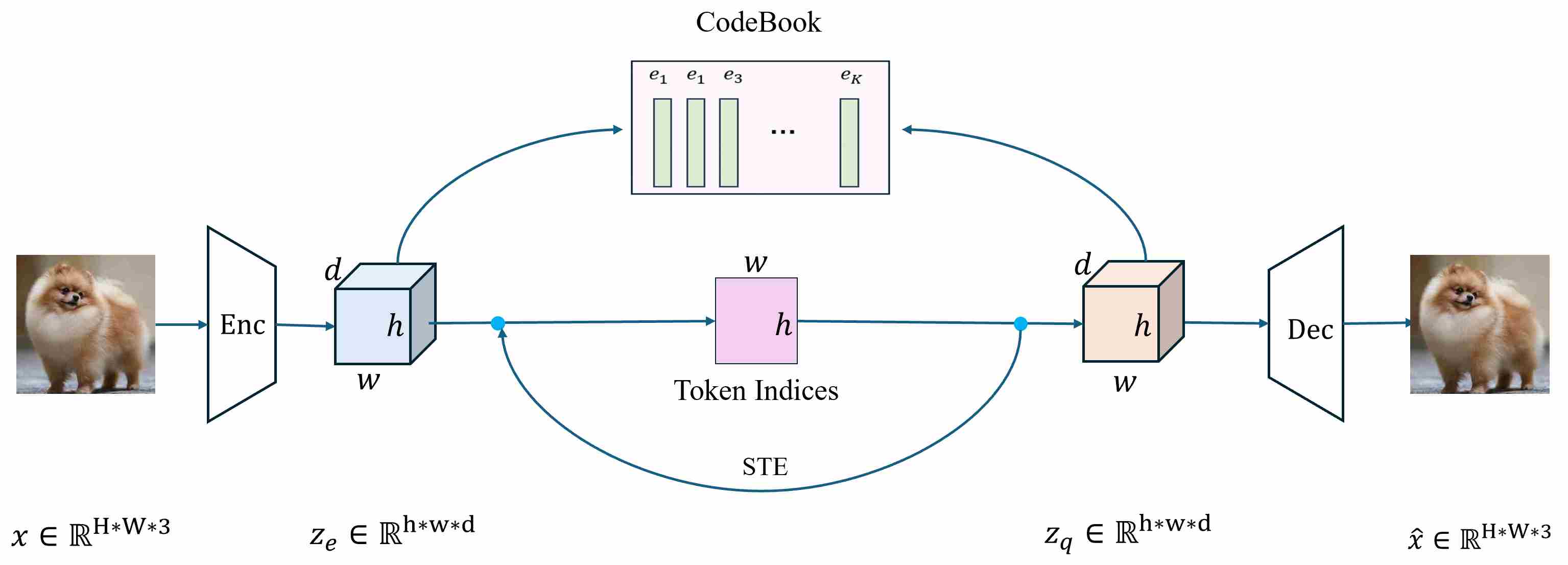
3.1 Vector Quantization: Foundations
Vector-Quantized VAE (VQ-VAE) preserves the overall encoder–decoder backbone but replaces the continuous latent variable with a discrete codebook indexing mechanism. Concretely, the encoder produces continuous embeddings \(z_e(x)\), which are then mapped to the nearest entry in a learnable codebook \(\{e_k\}_{k=1}^{K}\) by vector quantization:
\[k(x)=\arg\min_{j}\|z_e(x)-e_j\|_2,\qquad z_q(x)=e_{k(x)}.\]The decoder conditions on \(z_q(x)\) to reconstruct $x$. Accordingly, a canonical VQ-VAE architecture can be summarized as Encoder → Quantizer (codebook lookup) → Decoder, where the quantizer converts continuous encoder outputs into discrete indices (often viewed as “visual tokens” once flattened into a sequence).
3.2 The Advantage of Vector-Quantized
The introduction of a learned codebook in VQ-VAE brings two major advantages.
First, by replacing the continuous latent variable with a discrete code index selected via nearest-neighbor quantization, VQ-VAE largely removes the KL-driven posterior-to-prior matching pressure that is central to the standard VAE objective.
A useful probabilistic interpretation is to view $k$ as the latent variable with (i) a uniform prior \(p(k)=1/K\), and (ii) a deterministic (one-hot) posterior induced by quantization,
\[q_\phi(k\mid x)=\delta\big(k=k(x)\big).\]Under these assumptions, the KL term in a discrete-latent ELBO becomes a constant:
\[\mathrm{KL}(q_\phi(k\mid x)\,|\,p(k)) = \sum_{k} q_\phi(k\mid x)\log\frac{q_\phi(k\mid x)}{p(k)} = \log K,\]which is independent of $x$ and therefore can be dropped without changing the optimizer’s argmax. Consequently, the tokenizer training stage of VQ-VAE is not driven by a KL force that explicitly matches the posterior to a fixed prior, removing the canonical mechanism that causes VAEs with powerful decoders to collapse. In practice, VQ-VAE is trained with a reconstruction term plus vector-quantization-specific auxiliary losses (e.g., codebook and commitment terms, often with straight-through estimation), rather than the continuous VAE’s KL-regularized ELBO.
\[\mathcal{L} = \log p_\theta(x|z_q(x)) + \| \mathrm{sg}[z_e(x)] - e_k \|_2^2 + \beta \| z_e(x) - \mathrm{sg}[e_k]\|_2^2.\]Here \(\mathrm{sg}[\cdot]\) is the stop-gradient operator: identity in the forward pass, zero derivative in the backward pass. Reconstruction term \(\log p_\theta(x\mid z_q(x))\) trains the decoder, and via STE also trains the encoder to produce useful latents that decode well. Codebook (dictionary) loss \(\|\mathrm{sg}[z_e]-e_k\|^2\) pulls the selected code vector \(e_k\) toward the encoder output \(z_e(x)\). Encoder is stopped; only codebook updates. Commitment loss \(\beta\|z_e-\mathrm{sg}[e_k]\|^2\) prevents the encoder from “chasing” different codes too aggressively and stabilizes training by encouraging the encoder outputs to stay near chosen embeddings.
Importantly, the “KL-is-constant” argument hinges on the uniform prior + deterministic posterior setup. If one instead learns a non-uniform prior $p_\psi(k)$ (e.g., an autoregressive prior over code indices), then
$$ \mathrm{KL}(q_\phi(k\mid x)\,|\,p_\psi(k)) = -\log p_\psi(k(x)) + \text{const}, $$so the KL is no longer constant and becomes equivalent (up to a constant) to training the prior to assign high probability to the selected codes. This is consistent with the common two-stage recipe: first train the VQ-VAE tokenizer (reconstruction + quantization losses), and then fit a separate prior over the resulting discrete token sequences.
Second, discrete codes provide a natural interface for expressive learned priors. Instead of relying on a simple factorized Gaussian prior often used in baseline VAEs, VQ-VAE enables modeling the prior over discrete code indices \(p_\psi(k)\) with high-capacity autoregressive models (e.g., PixelCNN or Transformers) trained directly on token grids/sequences.
In practice, this two-stage recipe—(i) learning a high-fidelity tokenizer (encoder–quantizer–decoder) and (ii) fitting a strong autoregressive prior over the resulting discrete tokens—often yields markedly improved sample quality, capturing long-range structure and global coherence more effectively than simple continuous priors.
3.3 The Disadvantage of Vector-Quantized
Despite its advantages, VQ-VAE introduces a new set of challenges that are specific to codebook-based discretization.
Codebook collapse / dead codes: only a small subset of codebook entries may be selected during training, leaving many embeddings unused and effectively “dead,” which reduces representational capacity and harms reconstruction and downstream generation.
Index collapse and low code utilization: even when the codebook itself is large, the empirical distribution of selected indices can become highly imbalanced (e.g., dominated by a few frequent codes), leading to poor effective bitrate and limited diversity of discrete latents.
Optimization instability: the quantization step is non-differentiable, and training typically relies on straight-through estimators plus auxiliary objectives (e.g., commitment and codebook losses) or EMA updates; these ingredients can make optimization sensitive to hyperparameters and learning dynamics, sometimes yielding unstable convergence or degraded fidelity.
3.4 Root Causes of Codebook Learning Instability
Training Vector Quantization models is notoriously unstable. This instability stems from a fundamental conflict between the continuous nature of gradient-based optimization and the discrete nature of the quantization bottleneck. We can attribute the difficulty to three distinct but interrelated mechanisms:
3.4.1 The Non-Differentiable Argmin and the STE Approximation Gap
The most immediate hurdle in VQ training is that the quantization operation is mathematically non-differentiable: In the forward pass, the encoder outputs a continuous vector $z_e(x)$. The quantizer then maps this to the nearest codebook vector $e_k$ via a discrete argmin operation:
\[z_q(x) = e_k \quad \text{where} \quad k = \arg \min_j \|z_e(x) - e_j\|_2\]The Problem: Strictly speaking, the gradient of the quantization operation with respect to the encoder output is zero almost everywhere (since it is a piecewise constant step function).
\[\frac{\partial z_q}{\partial z_e} = 0\]If we used the true gradient, the encoder would receive no error signal, and learning would stall immediately.
The Flaw of STE (Straight-Through Estimator): To bypass this, we employ the Straight-Through Estimator. We manually define the gradient during the backward pass as an identity function, copying the gradients from the decoder inputs directly to the encoder outputs:
\[\frac{\partial \mathcal{L}}{\partial z_e} \approx \frac{\partial \mathcal{L}}{\partial z_q}\]Deep Analysis - The “Gradient Mismatch”: This is not the true gradient of the discrete objective; it is a biased surrogate. Bias matters because small changes in $z_e$ can cause sudden changes in $k$ (hard switching across Voronoi boundaries), yet STE supplies a smooth gradient signal as if no switching occurred. This gradient mismatch is a direct source of instability, oscillation, and failure to properly coordinate encoder/codebook updates.
3.4.2 Sparse Gradients and Codebook Collapse
Even if we accept STE for the encoder, the codebook itself is updated in a highly uneven way. Under hard assignment, only the selected code \(e_{k^*}\) receives a learning signal from a given latent. You can see this directly from the codebook loss term
\[\|\mathrm{sg}[z_e]-z_q\|_2^2 = \|\mathrm{sg}[z_e]-e_{k^*}\|_2^2.\]The gradient with respect to code $e_j$ is
\[\frac{\partial}{\partial e_j}\| \mathrm{sg}[z_e]-e_{k^*}\|_2^2 = 2\,(e_{k^*}-\mathrm{sg}[z_e])\cdot \mathbf{1}[j=k^*].\]So for all non-chosen codes \(j\neq k^*\), the gradient is exactly zero. In expectation over data, the magnitude of updates to a code \(e_j\) scales with how often it is selected:
\[\mathbb{E}[\Delta e_j] \propto \Pr(k^*=j)\cdot \mathbb{E}[\,e_j - z_e \mid k^*=j\,].\]If $\Pr(k^*=j)$ becomes tiny early in training, $e_j$ is essentially starved of updates and becomes a dead code. This creates a “Rich-Get-Richer” Dynamics:
- A few codes initially happen to be closer to the encoder outputs → they win assignments more often.
- Those codes get more updates → they move closer to dense regions of $z_e$.
- They become even more likely to win → assignments become increasingly concentrated.
This “winner-take-all” mechanism is one of the main reasons why VQ codebooks exhibit low utilization, skewed token histograms, and collapse to a small subset of codes, especially when $K$ is large or the encoder distribution shifts rapidly.
3.4.3 Encoder and codebook must co-adapt on different timescales
The final challenge lies in the complex training dynamics between the Encoder and the Codebook. They must be optimized simultaneously, but their objectives can conflict.
The Mechanism: The standard VQ loss function includes two auxiliary terms to govern this relationship ($sg$ denotes the stop-gradient operator):
\[\mathcal{L}_{VQ} = \underbrace{\| sg[z_e] - e \|_2^2}_{\text{Codebook Loss}} + \beta \underbrace{\| z_e - sg[e] \|_2^2}_{\text{Commitment Loss}}\]Deep Analysis - The “Cat and Mouse” Oscillation:
- Codebook Loss: Forces the codebook vectors to move toward the encoder outputs.
- Commitment Loss: Forces the encoder outputs to “commit” (stay close) to the current codebook vectors.
- Desynchronization:
- If the codebook updates too slowly (or the encoder moves too fast), the encoder outputs $z_e$ will constantly shift to new areas of the latent space before the codebook can settle. The codebook ends up chasing a moving target.
- If the commitment penalty $\beta$ is too high, the encoder is constrained and cannot explore the latent space to find better representations.
- If $\beta$ is too low, the encoder output variance becomes unbounded, making the training diverge.
Result: This leads to oscillation where neither component converges to a stable state, preventing the model from learning a consistent semantic mapping. Modern techniques like EMA (Exponential Moving Average) updates are specifically designed to fix this by forcing the codebook to smoothly follow the encoder statistics, rather than competing via gradient descent.
4. Codebook Update Dynamics
A healthy VQ model is not just about having a large codebook—it is about maintaining a stable, well-populated, and semantically meaningful partition of latent space throughout training. In practice, many VQ failures (dead codes, collapse, oscillation) are dynamical: they arise from how the codebook is updated over time, how fast it tracks the encoder, and how we intervene when some codes stop receiving assignments.
This section focuses on the “life cycle” of codes—how to update them, how to detect starvation, and how to revive or rebalance them.
4.1 EMA codebook updates
Let the encoder output a grid of latent vectors \(z_e \in \mathbb{R}^{H\times W \times D}\). For each position $i$ (flattening spatial indices), hard assignment selects
\[k_i = \arg\min_{k\in{1,\dots,K}} \|z_e^{(i)} - e_k\|_2^2\quad \Longrightarrow \quad z_q^{(i)} = e_{k_i}.\]Instead of updating $e_k$ via gradient descent (codebook loss), many implementations treat codebook learning as online clustering. Define per-code counts and sums over a minibatch:
\[n_k = \sum_i \mathbf{1}[k_i = k],\qquad m_k = \sum_i \mathbf{1}[k_i = k]\; z_e^{(i)}.\]Maintain exponential moving averages:
\[N_k \leftarrow \gamma N_k + (1-\gamma)n_k,\qquad M_k \leftarrow \gamma M_k + (1-\gamma)m_k,\]and update the embedding:
\[e_k \leftarrow \frac{M_k}{N_k + \varepsilon}.\]You can view this as tracking the centroid of the encoder outputs assigned to each code, with inertia controlled by $\gamma$.
Generally, EMA codebook update decouples codebook stability from optimizer quirks, makes codebook updates behave like smooth prototype tracking, and behaves like an online k-means, which matches the nearest-neighbor assignment semantics.
4.2 Reseeding / Restart of Under-used Codes
Even with EMA, some codes inevitably become under-used—especially early in training, or when $K$ is large. The key idea is to treat dead codes as a resource allocation problem: if a code receives no assignments, it is not participating in the representation and should be “reintroduced” near the data distribution.
we first detect dead or dying codes by tracking one or more indicators:
- usage count $N_k$ (EMA count) below a threshold,
- time since last assignment (in steps),
- effective vocabulary / perplexity over recent batches,
- assignment histogram entropy.
A simple rule:
\[\text{dead}(k) \;\; \Leftrightarrow \;\; N_k < \tau \quad \text{(for many steps)}.\]Some common reseeding strategies including but not limit to
Random reseed from current latents Pick a random latent vector from the current batch (or a buffer of recent latents) and set
\[e_k \leftarrow z_e^{(j)} + \sigma \epsilon,\quad \epsilon\sim \mathcal{N}(0,I).\]This places the code directly on the data manifold (plus small noise to avoid duplicates).
Hard-example reseed (high quantization error) Compute per-latent quantization error
\[\delta^{(i)} = \|z_e^{(i)} - e_{k_i}\|_2^2.\]Then reseed dead codes using latents with large \(\delta^{(i)}\), because they indicate regions not well covered by the existing codebook:
\[e_k \leftarrow z_e^{(i^*)}\quad \text{where } i^*=\arg\max_i \delta^{(i)} \text{ (or sample from top-(p\%))}.\]Split-and-perturb from popular codes If usage is heavily skewed, duplicate a frequently used code and perturb it:
\[e_{k_{dead}} \leftarrow e_{k_{popular}} + \sigma \epsilon.\]This is analogous to cluster splitting in k-means and can improve coverage of dense regions.
Reservoir buffer reseed Maintain a FIFO/reservoir of recent encoder latents \(\mathcal{B}={z_e}\). Reseed dead codes from \(\mathcal{B}\) to avoid dependence on a single batch.
5. Codebook Initialization Design
At the start of training, the encoder distribution \(p_\phi(z_e)\) is not yet well-shaped, and assignments are extremely sensitive to where code vectors ${e_k}$ sit. With random initialization, many codes are far from the support of $z_e$, hence they are never selected:
\[\Pr(k^*(z_e)=k) \approx 0 \quad \Rightarrow \quad \Delta e_k \approx 0,\]creating an absorbing “dead code” state. Since only selected codes get updated, early random advantages quickly amplify into long-term imbalance.
A good initialization aims to place code vectors close to the empirical latent distribution so that, already in the first few thousand steps,
\[\Pr(k^*(z_e)=k) > 0 \;\;\text{for most } k,\]which strongly improves utilization and stability. Some common initialization strategies including but not limit to
Random initialization (baseline) and its failure mode. The simplest baseline is
\[e_k \sim \mathcal{N}(0,\sigma^2 I)\quad \text{or}\quad e_k\sim \text{Unif}[-a,a].\]This works only when the scale roughly matches $z_e$. If the encoder output scale differs (common early on), the effective distances \(\| z_e-e_k\|_2^2\) are dominated by code magnitudes rather than data geometry, causing a small set of codes to win almost all assignments. This often manifests as low perplexity within the first epoch.
K-means seeding on early latents (offline / warm-start). A standard “data-driven” alternative is to run k-means on a latent sample pool:
First, collect a set of encoder outputs from a burn-in stage:
\[\mathcal{Z}=\{z_e^{(i)}\}_{i=1}^N,\quad z_e^{(i)}=E_\phi(x^{(i)}),\]Then, run k-means to obtain cluster centers \(\{\mu_k\}_{k=1}^K\):
\[\mu_k = \arg\min_{ \mu_k } \sum_{i=1}^N \min_k \|z_e^{(i)}-\mu_k\|_2^2,\]Finally, initialize codebook as \(e_k \leftarrow \mu_k.\)
Why it helps: k-means explicitly minimizes the same squared-distance objective that VQ uses for assignment, so it aligns codebook geometry with the encoder distribution from the start. It reduces the chance that any code lies completely off-manifold, hence reduces early dead codes and improves initial utilization/perplexity.
Online / streaming initialization (codebook “bootstrapping”). Instead of an explicit k-means pass, you can bootstrap codes online as training proceeds, especially useful for large $K$. The idea is: when a code is uninitialized or under-used, replace it with a representative latent from recent batches.
Let \(\mathcal{B}\) be a buffer of recent latents. For codes with low assignment count \(N_k\), do:
\[e_k \leftarrow z_e^{(j)}\quad \text{where } z_e^{(j)}\sim \mathcal{B}.\]Optionally add small noise:
\[e_k \leftarrow z_e^{(j)} + \sigma\epsilon,\quad \epsilon\sim\mathcal{N}(0,I).\]This can be viewed as a lightweight approximation to k-means where “cluster centers” are continuously refreshed from the latent stream. In EMA-based training, it integrates naturally: if \(N_k\) stays near zero, reseeding is essentially an online initialization.
Error-driven initialization (covering poorly represented regions). A more targeted online scheme uses the quantization residual to locate under-covered regions:
\[\delta^{(i)} = \|z_e^{(i)} - e_{k_i}\|_2^2.\]Select a latent with large residual and initialize/reseed a dead code with it:
\[e_k \leftarrow z_e^{(i^*)},\quad i^*\sim \text{Top-p selection} \text{ of } {\delta^{(i)}}.\]Intuition: large residuals indicate that existing codes do not cover that region well, so placing a code there increases coverage and utilization.
Feature-based initialization (pretrained latent spaces). When available, you can initialize the encoder (or a projection head) from a pretrained backbone, then seed the codebook on those more meaningful latents. Formally, if
\[z_e = P(E_{\text{pre}}(x)),\]then k-means/online seeding over these latents tends to yield more semantically structured codes and avoids early collapse driven by random encoder noise.
6. Objective function Design for Higher Utilization and Diversity
While the architectural improvements and update strategies (such as EMA) address the mechanics of quantization, the objective function serves as the guiding signal for the entire optimization process. The standard VQ-VAE loss formulation
\[\mathcal{L}_{\text{VQ}} = \underbrace{\mathcal{L}_{\text{rec}}(x, \hat{x})}_{\text{Reconstruction}} + \underbrace{\| \text{sg}[z_e(x)] - e \|_2^2}_{\text{Codebook Alignment}} + \underbrace{\beta \| z_e(x) - \text{sg}[e] \|_2^2}_{\text{Commitment}},\]is often insufficient to prevent codebook collapse or ensure high perceptual quality. This section details the evolution of loss functions designed to enforce codebook utilization, stabilize training dynamics, and improve reconstruction fidelity.
6.1 Entropy Regularization: Combating Codebook Collapse
In codebook-based VQ tokenizers, entropy regularization typically refers to adding an explicit objective that encourages high and balanced code usage, thereby mitigating dead codes, codebook collapse, and the resulting training instability. This is a training regularizer on the discrete bottleneck statistics—not “entropy coding” in the compression sense. Representative algorithms include Reg-VQ 31, GigaTok 32.
Assume a codebook of size $K$. For a minibatch, after quantization we obtain discrete indices
\[\{a_i\}_{i=1}^{M},\qquad a_i\in{1,\dots,K},\]where $M$ counts all assignments (batch $\times$ spatial locations). Define the empirical usage distribution (a histogram over codes):
\[p_k=\frac{1}{M}\sum_{i=1}^{M}\mathbf{1}[a_i=k].\]Its entropy is
\[H(p)=-\sum_{k=1}^{K} p_k\log(p_k+\varepsilon).\]Then, a standard entropy regularizer is simply
\[\mathcal{L}_{\text{ent}} = -H(p),\]i.e., minimizing \(\mathcal{L}_{\text{ent}}\) increases \(H(p)\), discouraging a peaked usage distribution. Equivalently, many papers write a KL-to-uniform penalty:
\[\mathcal{L}_{\text{prior}}=\mathrm{KL}(p\ \mid \ u)=\sum_{k=1}^{K} p_k\log\frac{p_k}{1/K} = \log K - H(p),\]where \(u_k=1/{K}\) is the uniform prior. Minimizing \(\mathrm{KL}(p\mid u)\) is exactly maximizing \(H(p)\) up to the constant \(\log K\). Reg-VQ 31 explicitly adopts this view as a prior distribution regularization to improve codebook utilization.
Intuition. Without this pressure, nearest-neighbor assignments create a “winner-take-all” dynamic: a small subset of codes gets selected early, receives most updates, and keeps winning—while many codes become inactive. Entropy/KL-to-uniform directly counteracts this by rewarding broader usage.
However, if \(p_k\) is computed from hard indices \(a_i=\arg\min_k\|z_i-e_k\|^2\), then the histogram is not differentiable with respect to the encoder outputs. In practice, entropy regularization is implemented through one of the following differentiable surrogates: soft Assignment Entropy is the most common and clean way to implement. Replace hard assignment by a soft distribution over codes:
\[\pi_{ik}=\mathrm{softmax}\!\left(-\frac{\|z_i-e_k\|^2}{\tau}\right), \qquad \bar p_k=\frac{1}{M}\sum_{i=1}^{M}\pi_{ik}.\]Then compute entropy or KL using \(\bar p\)
\[\mathcal{L}_{\text{ent}}^{\text{soft}} = -H(\bar p) = -\sum_{k=1}^{K} {\bar p}_k\log({\bar p}_k+\varepsilon).\]This makes the regularizer differentiable and allows gradients to shape \(z_e\) (and sometimes $e_k$).
6.2 Perceptual and Adversarial Losses
Traditional MSE loss ($\mathcal{L}_{2}$) assumes pixel independence and tends to produce blurry results. Blurry reconstructions allow the model to cheat by using a small set of “average” codes, indirectly contributing to low utilization. VQGAN 3 revolutionized this by introducing Perceptual and Adversarial losses.
6.2.1 Perceptual loss
Perceptual loss introduces in the context of style transfer and super-resolution, measures differences in feature space rather than pixel space. Let $\phi_l(\cdot)$ denote the feature map extracted from layer $l$ of a pretrained network (typically VGG-16 or VGG-19):
\[\mathcal{L}_{\text{perceptual}} = \sum_{l \in \mathcal{S}} \lambda_l \|\phi_l(\mathbf{x}) - \phi_l(\hat{\mathbf{x}})\|_2^2\]where $\mathcal{S}$ is a set of selected layers and $\lambda_l$ are layer-specific weights.
LPIPS (Learned Perceptual Image Patch Similarity) extends this by learning weights that correlate with human perceptual judgments:
\[\mathcal{L}_{\text{LPIPS}} = \sum_{l} \frac{1}{H_l W_l} \sum_{h,w} \|w_l \odot (\phi_l^{hw}(\mathbf{x}) - \phi_l^{hw}(\hat{\mathbf{x}}))\|_2^2\]where $w_l$ are learned channel-wise weights and $\phi_l^{hw}$ denotes the feature at spatial location $(h,w)$.
Benefit for VQ training: Perceptual loss provides more informative gradients that are less sensitive to exact quantization boundaries, partially mitigating STE error accumulation (Root Cause 1).
6.2.2 Adversarial Loss
Adversarial training introduces a discriminator $D_\psi$ that distinguishes real images from reconstructions:
Non-saturating GAN loss:
\[\mathcal{L}_{\text{G}} = -\mathbb{E}_{\mathbf{x}}[\log D_\psi(\hat{\mathbf{x}})]\] \[\mathcal{L}_{\text{D}} = -\mathbb{E}_{\mathbf{x}}[\log D_\psi(\mathbf{x})] - \mathbb{E}_{\mathbf{x}}[\log(1 - D_\psi(\hat{\mathbf{x}}))]\]Hinge loss formulation (commonly used in VQGAN):
\[\mathcal{L}_{\text{G}} = -\mathbb{E}_{\mathbf{x}}[D_\psi(\hat{\mathbf{x}})]\] \[\mathcal{L}_{\text{D}} = \mathbb{E}_{\mathbf{x}}[\max(0, 1 - D_\psi(\mathbf{x}))] + \mathbb{E}_{\mathbf{x}}[\max(0, 1 + D_\psi(\hat{\mathbf{x}}))]\]PatchGAN discriminator operates on local patches rather than the full image, providing spatially dense feedback:
\[\mathcal{L}_{\text{G}}^{\text{patch}} = -\mathbb{E}_{\mathbf{x}}\left[\frac{1}{|\mathcal{P}|}\sum_{p \in \mathcal{P}} D_\psi^{(p)}(\hat{\mathbf{x}})\right]\]where $\mathcal{P}$ indexes spatial patches.
Adaptive weight scheduling: VQGAN introduces an adaptive weight $\lambda_{\text{adv}}$ to balance reconstruction and adversarial losses:
\[\lambda_{\text{adv}} = \frac{\nabla_{G_L}[\mathcal{L}_{\text{recon}}]}{\nabla_{G_L}[\mathcal{L}_{\text{G}}] + \epsilon}\]where $\nabla_{G_L}$ denotes the gradient with respect to the last decoder layer. This ensures neither loss dominates during training.
6.2.3 Combined Reconstruction Objective
The complete reconstruction loss in modern VQ models (e.g., VQGAN) combines all components:
\[\mathcal{L}_{\text{recon}} = \lambda_{\text{pixel}}\mathcal{L}_{\text{pixel}} + \lambda_{\text{perc}}\mathcal{L}_{\text{perceptual}} + \lambda_{\text{adv}}\mathcal{L}_{\text{G}}\]Typical values: $\lambda_{\text{pixel}} = 1.0$, $\lambda_{\text{perc}} = 0.1 \sim 1.0$, $\lambda_{\text{adv}} = 0.1 \sim 0.5$ (or adaptively computed).
6.3 Codebook Geometry Regularization: Keep Codes Spread and Well-Behaved
Even if token usage is balanced, code vectors can crowd into a small region of latent space, making assignments brittle. Loss-level geometry regularizers address this by shaping \({e_k}\).
6.3.1 Norm control (scale stabilization)
Code norms can drift; a simple penalty is
\[\mathcal{R}_{\text{norm}}=\sum_k (\|e_k\|_2-1)^2,\]or explicit normalization \(e_k \leftarrow e_k/\|e_k\|\) (an implicit regularizer).
6.3.2 Diversity and Repulsion
A soft repulsion discourages code crowding:
\[\mathcal{R}_{\text{rep}}=\sum_{i\neq j}\exp\!\left(-\frac{\|e_i-e_j\|_2^2}{\tau}\right).\]Alternatively, one can regularize the code covariance or encourage orthogonality (stronger but sometimes over-constraining).
These terms are especially useful when collapse manifests as many codes becoming nearly identical.
6.4 Diversity-Promoting Losses
Beyond entropy, additional losses can explicitly encourage codebook diversity.
6.4.1 Codebook Orthogonality Loss
Encouraging codebook entries to be mutually orthogonal prevents clustering:
\[\mathcal{L}_{\text{ortho}} = \|\mathbf{E}^T\mathbf{E} - \mathbf{I}\|_F^2\]where $\mathbf{E} \in \mathbb{R}^{K \times D}$ is the codebook matrix and $|\cdot|_F$ is the Frobenius norm.
For L2-normalized codebook entries $\tilde{\mathbf{E}}$:
\[\mathcal{L}_{\text{ortho}}^{\text{norm}} = \sum_{i \neq j} (\tilde{e}_i \cdot \tilde{e}_j)^2\]This penalizes high cosine similarity between different codes.
6.4.2 Codebook Variance Loss
Encouraging spread in the codebook:
\[\mathcal{L}_{\text{var}} = \max\left(0, \gamma - \text{Var}[\{e_k\}_{k=1}^K]\right)\]where $\gamma$ is a target variance threshold. This prevents codes from clustering in a small region.
6.4.3 Contrastive Codebook Loss
Drawing inspiration from contrastive learning, we can treat codes as classes:
\[\mathcal{L}_{\text{contrast}} = -\log \frac{\exp(\mathbf{z}_e \cdot \mathbf{z}_q / \tau)}{\sum_{k=1}^{K} \exp(\mathbf{z}_e \cdot e_k / \tau)}\]This InfoNCE-style loss encourages each encoder output to be close to its assigned code and far from others, promoting well-separated codebook entries.
6.4.4 Variance-Invariance-Covariance regularization
Adapting the Variance-Invariance-Covariance regularization 33 to codebooks:
Variance term (prevent collapse):
\[\mathcal{L}_{\text{vic-var}} = \frac{1}{D}\sum_{d=1}^{D} \max(0, \gamma - \sqrt{\text{Var}[e_{:,d}] + \epsilon})\]Covariance term (decorrelate dimensions):
\[\mathcal{L}_{\text{vic-cov}} = \frac{1}{D}\sum_{i \neq j} [\text{Cov}(\mathbf{E})]_{ij}^2\]Combined:
\[\mathcal{L}_{\text{VICReg}} = \lambda_v \mathcal{L}_{\text{vic-var}} + \lambda_c \mathcal{L}_{\text{vic-cov}}\]7. Codebook Architecture Design
The above sections (section 4, section 5, and section 6) show how to improve codebook quality by updating dynamics (EMA, restarts, initialization) and objectives design. A third, largely orthogonal axis is to redesign the parameterization of the discrete space itself: instead of a single monolithic codebook $\mathbf{E}\in\mathbb{R}^{K\times D}$, we construct structured, compositional, or hierarchical codebooks that represent each latent vector using multiple smaller codebooks and a composition rule.
Concretely, recall standard VQ at token position $i$:
\[k_i=\arg\min_{k\in{1,\dots,K}}\|z_e^{(i)}-e_k\|_2^2,\quad z_q^{(i)}=e_{k_i}.\]In structured codebooks, we introduce $M$ codebooks \(\{\mathbf{E}^{(m)}\}_{m=1}^M\) and encode each token by a tuple of indices
\[\mathbf{k}_i = \big(k_i^{(1)},\dots,k_i^{(M)}\big),\quad k_i^{(m)}\in{1,\dots,K_m},\]then construct the quantized embedding via a composition operator $g(\cdot)$:
\[z_q^{(i)} = g\!\left(e_{k_i^{(1)}}^{(1)},\dots,e_{k_i^{(M)}}^{(M)}\right).\]This family includes Residual Quantization (RVQ/RQ), Group/Split VQ (Product Quantization), Multi-Head / Multi-Codebook VQ, Factorized Codes, and Hierarchical / Multi-Scale VQ. The shared motivation is:
- Increase effective vocabulary without a giant matrix. A single huge $K$ often collapses (many dead codes) because only a small fraction gets assignments. Splitting into multiple smaller codebooks makes each sub-codebook easier to populate and update.
- Make nearest-neighbor search better-conditioned. High-dimensional nearest-neighbor assignment over a massive codebook is brittle; multiple smaller assignments are often more stable.
- Expose a rate–distortion knob. Many structured designs allow progressive refinement (residual stages, coarse-to-fine levels), naturally supporting variable bitrate / token budget control.
Below we summarize the dominant architectural patterns.
7.1 Residual Quantization (RVQ / RQ-style VQ)
Idea. Quantize a vector by successively quantizing residual errors, so one token becomes a stack of code indices that progressively refines reconstruction.
Let $r^{(0)} = z_e^{(i)}$. For stage $m=1,\dots,M$:
\[k_i^{(m)} =\arg\min_{k}\|r^{(m-1)}-e_k^{(m)}\|_2^2,\]where
\[q^{(m)} =e_{k_i^{(m)}}^{(m)}, \qquad r^{(m)} =r^{(m-1)}-q^{(m)}.\]The final quantized embedding is additive:
\[z_q^{(i)}=\sum_{m=1}^{M} q^{(m)}.\]Why it helps stability. Early stages capture coarse structure and receive strong gradients/assignments; later stages refine details. Compared to “one-shot” huge-$K$ VQ, each stage has a smaller search space and tends to maintain higher utilization (especially if residual stages are encouraged not to die).
Typical failure mode. Later stages can become under-used (all residuals mapped to a small subset). In practice, this is where stability techniques still matter: EMA updates per stage, reseeding per stage, and entropy/diversity regularization on each sub-codebook.
Representative: RQ-VAE / residual-quantized AR pipelines for high-res image generation 9.
7.2 Group / Split VQ and Product Quantization (PQ-style VQ)
Idea. Split the latent channel dimension into groups and quantize each group independently, turning one code into a Cartesian product of subcodes.
Split:
\[z_e^{(i)}=\big[z_e^{(i,1)}\;\dots\;z_e^{(i,G)}\big],\quad z_e^{(i,g)}\in\mathbb{R}^{D_g},\ \sum_g D_g=D.\]For each group:
\[k_i^{(g)}=\arg\min_{k}\|z_e^{(i,g)}-e_k^{(g)}\|_2^2,\quad z_q^{(i,g)}=e*{k_i^{(g)}}^{(g)}.\]Compose by concatenation:
\[z_q^{(i)}=\big[z_q^{(i,1)},\;\dots\;,z_q^{(i,G)}\big],\](optionally followed by a projection layer if you want to map back to a fixed $D$).
Effective capacity. If each group has $K$ entries, the number of possible joint codes is $K^G$ (combinatorial explosion), while each sub-problem stays small. This is the classic Product Quantization principle.
Why it helps. Each sub-codebook sees many assignments (because every token uses every group), which often reduces dead codes and improves utilization compared to one giant codebook.
Representative in modern tokenizers: Imagefolder 34 uses dual-branch product quantization to boost representation power without increasing token length.
7.3 Multi-Head / Multi-Codebook Quantization (Parallel composition)
Idea. Instead of splitting channels directly, create multiple “views” (heads) of the same latent, quantize each with its own codebook, then compose.
A common form:
\[z_e^{(i,m)} = W_m z_e^{(i)},\quad z_q^{(i,m)}=Q^{(m)}(z_e^{(i,m)}),\quad z_q^{(i)} = g\big(z_q^{(i,1)},\dots,z_q^{(i,M)}\big),\]where $g$ can be concatenation or summation.
Why it helps. Heads/codebooks can specialize (texture vs shape, local vs global cues), and the model can avoid pushing all semantics into a single set of embeddings, which is a common driver of collapse.
Two recent patterns worth highlighting:
- Dual-codebook decoupling (semantic vs pixel). TokenFlow 35 explicitly decouples semantic and pixel-level representations with a dual-codebook design while keeping alignment through a shared mapping mechanism.
- Multi-codebook factorization for scalability. FQGAN 36 factorizes a large vocabulary into multiple independent sub-codebooks plus a disentanglement regularizer to reduce redundancy across sub-codebooks.
7.4 Hierarchical / Multi-Scale Codebooks
Idea. Quantize at multiple spatial resolutions (e.g., a coarse grid + a fine grid), each with its own codebook. This is hierarchical in space rather than in channel groups.
VQ-VAE-2 is the canonical example: a top-level latent \(z_e^{\text{top}}\in\mathbb{R}^{h_1\times w_1\times d_1}\) and a bottom-level latent \(z_e^{\text{bot}}\in\mathbb{R}^{h_2\times w_2\times d_2}\) are quantized separately:
\[z_q^{\text{top}}=Q_{\text{top}}(z_e^{\text{top}}),\quad z_q^{\text{bot}}=Q_{\text{bot}}(z_e^{\text{bot}}),\quad \hat{x}=D(z_q^{\text{top}}, z_q^{\text{bot}}).\]Why it helps. Coarse codes capture global structure with stable assignments; fine codes focus on local details. Hierarchy therefore reduces the burden on any single codebook to represent both “layout” and “texture”, improving both fidelity and code usage.
Representative: VQ-VAE-2 2.
7.5 Compact 1D Tokenization (TiTok & Pooling Architectures)
Traditional VQ-GANs preserve the 2D spatial grid (e.g., mapping a $256 \times 256$ image to a $16 \times 16$ token grid). This results in sequence lengths ($N=256$) that grow quadratically with image resolution, creating a bottleneck for LLMs.
Idea: Break the fixed correspondence between spatial patches and tokens. Map the 2D image feature grid to a compact 1D latent sequence of fixed size (e.g., 32 or 64 tokens), regardless of input resolution.
Mechanism (TiTok style):
- Encoder: Produces a standard 2D feature grid.
Pooler / Resampler: Uses a Perceiver-like attention block or adaptive pooling to compress the 2D grid into $N$ 1D latent vectors.
\[\text{Latents}_{1D} = \text{Attention}(Q=\text{LearnableQueries}, K=Z_{2D}, V=Z_{2D})\]- Quantization: Quantize the 1D vectors.
- Decoder: Reconstructs the 2D grid from 1D tokens (often conditioning on position embeddings) to generate the image.
Why it dominates: It decouples token count from image resolution. A $512 \times 512$ image can be represented by 64 tokens, making it feasible to interleave multiple high-res images in a single LLM context window without exploding compute costs.
8. Implicit / codebook-free quantizers
Implicit quantizers remove the explicit learned lookup table $E$. Instead, they define the discrete set \(\mathcal{C}\) via a quantization rule; the “effective vocabulary” often arises as a product space (scalar levels across channels) or a binary code space.
8.1 Finite Scalar Quantization (FSQ)
FSQ proposes replacing vector quantization with a simple scheme: project to a low-dimensional representation and quantize each dimension to a small set of fixed values, yielding an implicit codebook given by the product of these sets.
Let an encoder map an image/video $x$ to a latent grid
\[z_e(x)\in\mathbb{R}^{H\times W\times C}.\]FSQ typically introduces a learnable projection (often linear/MLP) to a lower-dimensional quantization space:
\[y(x) = \pi_\theta(z_e(x))\in\mathbb{R}^{H\times W\times d},\]where $d$ is the number of quantized channels (often much smaller than $C$). For each channel \(j\in \{1,\dots,d\}\), FSQ defines a fixed set of scalar levels \(\mathcal{L}_j\) (e.g., symmetric levels in ([-1,1])):
\[\mathcal{L}_j=\{\ell_{j,1},\ldots,\ell_{j,L_j}\}.\]The implicit codebook is then the product space
\[\mathcal{C} = \mathcal{L}_1\times\cdots\times\mathcal{L}_d,\]with effective cardinality \(\|\mathcal{C}\|=\prod_{j=1}^d L_j\). FSQ can be summarized as a simple continuous → discrete → continuous pipeline, where the actual discretization happens at the integer index step.
Range bounding (continuous). Take the encoder output \(z\) and squash it into a fixed bounded interval (commonly \([-1, 1]\)) using a function like \(\tanh\): \(u = \tanh(z)\). This is still floating-point and continuous.
Scale to a discrete grid (continuous → grid coordinates). For each dimension $d$, choose a finite number of levels $L_d$. Map \(u_d \in [-1,1]\) to grid coordinates in \([0, L_d-1]\):
\[s_d = \frac{u_d + 1}{2}\,(L_d - 1)\]Quantize to integer indices (discrete). Round to obtain the discrete integer index (the true “token” per dimension):
\[i_d = \mathrm{round}(s_d)\in \{0,\dots,L_{d}-1\}\]In training, gradients are typically passed using a straight-through estimator.
Dequantize back to a continuous value for the decoder (discrete → continuous). Convert each integer index back to a representative value on the bounded interval (a fixed grid point):
\[u^{(q)}_d = \frac{i_d}{L_d-1}\cdot 2 - 1\]This is “continuous” in type (float), but it can only take finite values per dimension.
(Optional) Pack indices into a single token id. The per-dimension indices \({i_d}\) can be combined into one integer token via mixed-radix encoding, yielding a vocabulary size \(\prod_d L_d\).
In short: Step 3 produces the discrete integers (tokens), while Step 4 is an implicit lookup (rule-based instead of a learned codebook) to produce a continuous tensor that the decoder can consume.
8.2 Lookup-Free Quantization (LFQ)
LFQ follows a similar continuous → discrete → (optional) continuous pattern, but it removes the learned embedding codebook lookup entirely. A minimal (binary) LFQ can be summarized as:
Start from a continuous latent (continuous). Let the encoder produce a latent vector \(z \in \mathbb{R}^{D}\) (or a feature map flattened into vectors). No nearest-neighbor search is performed.
Element-wise discrete quantization without lookup (discrete). Quantize each latent dimension independently using a simple rule (most commonly a binary sign threshold):
\[q = \mathrm{sign}(z) \in \{-1, +1\}^{D}\]Training typically uses a straight-through estimator so gradients can flow through this non-differentiable step.
Convert the discrete pattern to a token id (discrete indexing). Interpret the quantized vector as a discrete code and map it to an integer token id via a fixed “basis” (e.g., binary or mixed-radix encoding):
\[\text{token_id} = \sum_{d=0}^{D-1} b_d \, 2^d,\quad b_d=\mathbb{1}[q_d>0]\,\text{or}\, \mathbb{0}[q_d<=0]\]More generally, each dimension can be treated as a discrete variable and packed into one id with mixed-radix encoding.
(Optional) Represent the token for the decoder (no codebook table). Since there is no learned \(K\times D\) codebook to look up, the decoder can consume either:
- the quantized vector $q$ directly (as a continuous tensor with discrete values), or
- a fixed, rule-based mapping from ids back to a continuous representation (an implicit “lookup” defined by the encoding scheme rather than learned embeddings).
Encourage code utilization (regularization). To avoid degenerate codes (e.g., always the same sign pattern), LFQ commonly adds an entropy-style regularizer that pushes each discrete variable (bit) toward a balanced marginal distribution, improving “vocabulary usage.”
In short: LFQ discretizes by per-dimension thresholding (or small discrete alphabets) and packs the result into token ids, while avoiding nearest-neighbor search and avoiding a learned embedding codebook lookup—hence “lookup-free.”
8.3 Binary Spherical Quantization (BSQ)
BSQ can be summarized as a project → normalize → binarize → (back-)project pipeline, where the “codebook” is implicit (the corners of a hypercube on a unit sphere), so there is no learned $K\times D$ embedding table.
Encode to a continuous latent (continuous). The encoder produces a high-dimensional embedding: \(z = E(x)\in\mathbb{R}^d.\)
Project to a low-dimensional bottleneck (continuous). Apply a linear projection to a much smaller dimension \(L\ll d\):
\[v = \mathrm{Linear}(z)\in\mathbb{R}^L.\]Project onto the unit hypersphere (continuous, spherical normalization). Normalize to unit length:
\[u = \frac{v}{\lVert v\rVert}.\]Binary quantization on the sphere (discrete, per-dimension sign) Binarize each dimension using the sign function and keep the result on the unit sphere via a fixed scaling:
\[\hat u = \sqrt{\frac{1}{L}}\;\mathrm{sign}(u),\]with a convention \(\mathrm{sign}(0)\to 1\). For training, use a straight-through estimator (STE) to pass gradients:
\[\mathrm{sign}_{\mathrm{STE}}(x)=\mathrm{sg}(\mathrm{sign}(x)-x)+x.\]Back-project to the decoder latent space (continuous) Map the quantized spherical code back to (d) dimensions for the decoder:
\[\hat z = \mathrm{Linear}(\hat u)\in\mathbb{R}^d.\](Inference) Convert the binary pattern to a token id (discrete indexing) Assign a discrete token by interpreting the signs as bits (binary encoding):
\[k = \sum_{i=1}^{L}\mathbf{1}[v_i>0]\;2^{i-1}.\]
Why it’s “codebook-free” in practice: BSQ’s codebook is implicit:
\[C_{\text{BSQ}} = \left\{ -\sqrt{\tfrac{1}{L}},\;+\sqrt{\tfrac{1}{L}} \right\}^L\](the hypercube corners on the unit sphere), so you don’t store or search a learned embedding table—quantization is just normalize + sign.
9. References
van den Oord A, Vinyals O, Kavukcuoglu K. Neural Discrete Representation Learning [C]//Proceedings of the 31st International Conference on Neural Information Processing Systems (NeurIPS). 2017. ↩ ↩2
Razavi A, van den Oord A, Vinyals O. Generating Diverse High-Fidelity Images with VQ-VAE-2 [C]//Proceedings of the 33rd International Conference on Neural Information Processing Systems (NeurIPS). 2019. ↩ ↩2 ↩3
Esser P, Rombach R, Ommer B. Taming Transformers for High-Resolution Image Synthesis [C]//Proceedings of the IEEE/CVF Conference on Computer Vision and Pattern Recognition (CVPR). 2021: 12873-12883. ↩ ↩2 ↩3
Yu J, Li X, Koh J Y, et al. Vector-quantized Image Modeling with Improved VQGAN [C]//International Conference on Learning Representations (ICLR). 2022. ↩ ↩2
Mentzer F, Minnen D, Agustsson E, et al. Finite Scalar Quantization: VQ-VAE Made Simple [C]//International Conference on Learning Representations (ICLR). 2024. ↩
(Refers to MAGVIT-2) Yu L, Lezama J, Gundavarapu N B, et al. Language Model Beats Diffusion–Tokenizer is Key to Visual Generation [C]//International Conference on Learning Representations (ICLR). 2024. ↩
Zhao Y, Xiong Y, Krähenbühl P. Image and Video Tokenization with Binary Spherical Quantization [C]//Proceedings of the European Conference on Computer Vision (ECCV). 2024. ↩
Ramesh A, Pavlov M, Goh G, et al. Zero-Shot Text-to-Image Generation [C]//Proceedings of the 38th International Conference on Machine Learning (ICML). 2021. ↩
Lee D, Kim C, Kim S, et al. Autoregressive Image Generation using Residual Quantization [C]//Proceedings of the IEEE/CVF Conference on Computer Vision and Pattern Recognition (CVPR). 2022. ↩ ↩2
Chen M, Radford A, Child R, et al. Generative Pretraining from Pixels [C]//Proceedings of the 37th International Conference on Machine Learning (ICML). 2020. ↩
Bao H, Dong L, Piao S, et al. BEiT: BERT Pre-Training of Image Transformers [C]//International Conference on Learning Representations (ICLR). 2022. ↩
Dong X, Bao J, Chen D, et al. PeCo: Perceptual Codebook for BERT Pre-Training of Vision Transformers [C]//Proceedings of the AAAI Conference on Artificial Intelligence. 2023. ↩
Peng Z, Dong L, Bao H, et al. BEiT v2: Masked Image Modeling with Vector-Quantized Visual Tokenizers [J]. arXiv preprint arXiv:2208.06366, 2022. ↩
Wang W, Bao H, Dong L, et al. Image as a Foreign Language: BEiT Pretraining for Vision and Vision-Language Tasks [C]//Proceedings of the IEEE/CVF Conference on Computer Vision and Pattern Recognition (CVPR). 2023. ↩
Li Y, Mao H, Girshick R, et al. MAGE: MAsked Generative Encoder to Unify Representation Learning and Image Generation [C]//Proceedings of the IEEE/CVF Conference on Computer Vision and Pattern Recognition (CVPR). 2023. ↩
Chang H, Zhang H, Jiang L, et al. MaskGIT: Masked Generative Image Transformer [C]//Proceedings of the IEEE/CVF Conference on Computer Vision and Pattern Recognition (CVPR). 2022. ↩
Ge Y, Xu Y, Geng Z, et al. SEED: Semantic-Aligned Discrete Tokenizer for Vision-Language Models [C]//International Conference on Learning Representations (ICLR). 2024. ↩
Ge Y, Zhao S, Geng Z, et al. Making Llama 3 Blind: Unified Generation and Understanding for Multimodal LLMs (SEED-X) [J]. arXiv preprint arXiv:2404.14396, 2024. ↩
Jin Y, Xu K, Chen Y, et al. LaVIT: Unified Generation and Understanding for Vision-Language Models [C]//International Conference on Learning Representations (ICLR). 2024. ↩
Sun Q, Cui Y, Zhang X, et al. Generative Pretraining in Multimodality [C]//International Conference on Learning Representations (ICLR). 2024. ↩
Wang X, Zhang X, Sun Q, et al. Emu3: Next-Token Prediction is All You Need [J]. arXiv preprint arXiv:2409.18869, 2024. ↩
Chameleon Team. Chameleon: Mixed-Modal Early-Fusion Foundation Models [J]. arXiv preprint arXiv:2405.09818, 2024. ↩
Xie J, Wu Z, Wang Y, et al. Show-o: One Single Transformer to Unify Multimodal Understanding and Generation [J]. arXiv preprint arXiv:2408.12528, 2024. ↩
Wu C, Xia L, Shen Y, et al. Janus: Decoupling Visual Encoding for Unified Multimodal Understanding and Generation [J]. arXiv preprint arXiv:2410.13848, 2024. ↩
Sun P, Chen S, Zhang C, et al. Autoregressive Model Beats Diffusion: Llama for Scalable Image Generation [J]. arXiv preprint arXiv:2406.06525, 2024. ↩
Zhu Y, Wu J, Gao R, et al. Open-MAGVIT2: An Open-Source Project toward Democratizing Auto-regressive Visual Generation [J]. arXiv preprint arXiv:2409.04410, 2024. ↩
Yu Q, Guo G, Wang X, et al. TiTok: An Image is Worth 32 Tokens for Reconstruction and Generation [C]//Proceedings of the European Conference on Computer Vision (ECCV). 2024. ↩
Shi F, Luo Z, Ge Y, et al. Scalable image tokenization with index backpropagation quantization[C]//Proceedings of the IEEE/CVF International Conference on Computer Vision. 2025: 16037-16046. ↩
Kingma D P, Welling M. Auto-Encoding Variational Bayes [J]. arXiv preprint arXiv:1312.6114, 2013. ↩
Doersch C. Tutorial on Variational Autoencoders [J]. arXiv preprint arXiv:1606.05908, 2016. ↩
Zhang J, Zhan F, Theobalt C, et al. Regularized Vector Quantization for Tokenized Image Synthesis [C]//Proceedings of the IEEE/CVF Conference on Computer Vision and Pattern Recognition (CVPR). 2023. ↩ ↩2
Xiong T, Liew J H, Huang Z, et al. Gigatok: Scaling visual tokenizers to 3 billion parameters for autoregressive image generation[J]. arXiv preprint arXiv:2504.08736, 2025. ↩
Bardes A, Ponce J, LeCun Y. VICReg: Variance-Invariance-Covariance Regularization for Self-Supervised Learning [C]//International Conference on Learning Representations (ICLR). 2022. ↩
Li X, Qiu K, Chen H, et al. Imagefolder: Autoregressive image generation with folded tokens[J]. arXiv preprint arXiv:2410.01756, 2024. ↩
Qu L, Zhang H, Liu Y, et al. Tokenflow: Unified image tokenizer for multimodal understanding and generation[C]//Proceedings of the Computer Vision and Pattern Recognition Conference. 2025: 2545-2555. ↩
Bai Z, Gao J, Gao Z, et al. Factorized visual tokenization and generation[J]. arXiv preprint arXiv:2411.16681, 2024. ↩