Update Jan 10, 2026: This post has been summit to ICLR 2026 Blog Posts track

Inverse problems, which aim to recover a signal of interest from indirect and often corrupted measurements, are a cornerstone of computational science and engineering. These problems are typically ill-posed, necessitating the use of prior knowledge to regularize the solution space and ensure a unique and stable reconstruction. This post provides a structured exposition of the evolution of priors in solving inverse problems, from classical formulations to the modern paradigm of deep generative models. This work aims to bridge the conceptual gap between classical and modern techniques, offering a unified view of the role of priors in solving generative inverse problems.

1. The Probabilistic Formulation of Inverse Problems

An inverse problem seeks to recover an unknown signal $\mathbf{x} \in \mathbb{R}^n$ from a set of observed measurements $\mathbf{y} \in \mathbb{R}^m$. This process is typically modeled by a linear forward operator $\mathbf{A}: \mathbb{R}^n \rightarrow \mathbb{R}^m$ and corrupted by additive noise $\mathbf{n} \in \mathbb{R}^m$:

The operator $\mathbf{A}$ encodes the physics or geometry of the measurement process. For example:

• In image deblurring, $\mathbf{A}$ is a convolution with a blur kernel.
• In super-resolution or compressed sensing, $\mathbf{A}$ is a subsampling or projection operator.
• In computed tomography (CT), $\mathbf{A}$ is a (discretized) Radon transform.
• In magnetic resonance imaging (MRI), $\mathbf{A}$ corresponds to a subsampled Fourier transform.

Beyond imaging, similar formulations appear in audio denoising and deconvolution, geophysical exploration, astronomical imaging, and more generally in parameter estimation for scientific systems.

The problem is deemed “inverse” because we seek to reverse the effect of $\mathbf{A}$. It is often ill-posed, meaning that a solution may not exist, may not be unique, or may not depend continuously on the data. Depending on whether prior knowledge is provided, we divide the solution of inverse problems into two major categories for discussion.

1.1 Inverse Problems without Priors: Maximum Likelihood Estimation

In the absence of any prior knowledge about the signal $\mathbf{x}$, our estimation relies solely on the data formation model. A common and mathematically convenient assumption is that the noise $\mathbf{n}$ is independent and identically distributed (i.i.d.) Gaussian with zero mean and variance $\sigma^2$, i.e.,

This assumption allows us to formulate the problem within the framework of Maximum Likelihood Estimation (MLE). The likelihood function $p(\mathbf{y}\mid \mathbf{x})$ describes the probability of observing the measurements $\mathbf{y}$ given a specific signal $\mathbf{x}$. Under the Gaussian noise assumption, the relationship $\mathbf{y} = \mathbf{A}\mathbf{x} + \mathbf{n}$ implies that $\mathbf{y}$ is also Gaussian-distributed, centered at $\mathbf{A}\mathbf{x}$:

The probability density function for this multivariate Gaussian distribution is given by:

The MLE principle seeks the estimate $\hat{\mathbf{x}}_{\text{MLE}}$ that maximizes this likelihood. For computational stability and simplicity, it is standard practice to maximize the log-likelihood instead:

Since the first term is a constant with respect to $\mathbf{x}$, and maximizing the negative of a function is equivalent to minimizing the function itself, the MLE objective simplifies to a least-squares problem:

This objective is also known as the Mean Squared Error (MSE) data fidelity term. While principled, it is insufficient for ill-posed problems, as many different signals $\mathbf{x}$ can yield a similarly small residual \(\|\mathbf{y} - \mathbf{A}\mathbf{x}\|_2^2\), often resulting in solutions dominated by noise ^{1 2 3}.

1.2 Inverse Problems with Priors: Maximum A Posteriori Estimation

To overcome the limitations of MLE, we introduce prior knowledge about the expected properties of the signal $\mathbf{x}$. This is formalized using a Bayesian approach. We define a prior distribution $p(\mathbf{x})$ that assigns higher probability to signals that are plausible (e.g., natural images with smooth regions and sharp edges) and lower probability to others (e.g., pure noise).

Using Bayes’ theorem, we can combine the likelihood $p(\mathbf{y}\mid \mathbf{x})$ with the prior $p(\mathbf{x})$ to obtain the posterior distribution $p(\mathbf{x}\mid \mathbf{y})$:

The posterior represents our updated belief about $\mathbf{x}$ after observing the data $\mathbf{y}$. The goal of Maximum A Posteriori (MAP) estimation is to find the signal $\hat{\mathbf{x}}_{\text{MAP}}$ that maximizes this posterior probability ^{2 3}:

Since the denominator $p(\mathbf{y})$ is constant with respect to $\mathbf{x}$, the MAP objective becomes:

Again, we work with the log-posterior for convenience:

Substituting the log-likelihood term from the Gaussian noise model, we get:

This is equivalent to minimizing the negative log-posterior:

This formulation elegantly connects Bayesian inference to regularized optimization. If we define a regularization function $R(\mathbf{x}) = -\log p(\mathbf{x})$ and absorbing all constants into a free regularization weight $\lambda > 0$, the MAP estimation is precisely equivalent to solving the following optimization problem:

Here, the data fidelity term ensures consistency with the measurements, while the regularization term $R(\mathbf{x})$ enforces the prior. The choice of $R(\mathbf{x})$ is paramount and has been the subject of extensive research.

2. Classical Regularization with Non-Generative Priors

Before the widespread adoption of deep generative models, the regularization term $R(\mathbf{x})$ in the MAP objective was primarily designed based on handcrafted statistical assumptions about the signal.

These priors do not attempt to model the full high-dimensional distribution $p(\mathbf{x})$; instead, they encode specific structural properties—such as smoothness, sparsity, or non-local self-similarity—that are believed to hold for natural signals.

2.1 Smoothness Priors (Handcrafted Explicit Priors)

Core assumption: Natural signals, such as images, are predominantly smooth or piecewise-constant. High-frequency variations are often attributed to noise rather than the underlying signal structure. Representative Regularizers including:

1. Tikhonov Regularization ¹: This is one of the earliest and most fundamental regularizers, penalizing the L2-norm of the signal’s derivatives. From a Bayesian perspective, this corresponds to assuming a zero-mean Gaussian prior on the signal’s derivative, i.e.,

   \[p(\mathbf{L}\mathbf{x}) \propto \exp \left(- \| \mathbf{L}\mathbf{x} \|_2^2 / 2\tau^2\right)\,\Longrightarrow\,R(\mathbf{x}) = -\log p(\mathbf{L}\mathbf{x}) = \|\mathbf{L}\mathbf{x}\|_2^2\]

   where $\mathbf{L}$ is a linear operator, typically a finite-difference approximation of the gradient or Laplacian.

2. Total Variation (TV) ⁴: A significant advancement over Tikhonov, the TV regularizer is defined as the L1-norm of the signal’s gradient magnitude, this is equivalent to imposing a Laplacian prior on the gradient magnitudes, i.e.,

   \[p(\nabla \mathbf{x}) \propto \exp \left(- \|\nabla \mathbf{x}\|_1 / \tau\right)\,\Longrightarrow\,R(\mathbf{x}) = -\log p(\nabla \mathbf{x}) = \|\nabla \mathbf{x}\|_1\]

   Unlike the L2-norm, which penalizes large gradients heavily, the L1-norm promotes solutions where gradients are sparse, effectively preserving sharp edges while enforcing smoothness in flat regions.

2.2 Sparsity Priors in Transform Domains

Core assumption: While signals may not be sparse in their native domain (e.g., pixel space), they often admit a sparse representation in a suitable transform domain.

Let $\mathbf{\Psi}$ denote a transform (orthonormal basis, frame, or learned dictionary), and let \(\boldsymbol{\alpha} = \mathbf{\Psi}\mathbf{x}\) be the transform coefficients. Sparsity priors posit that most entries of $\boldsymbol{\alpha}$ are zero or near-zero. This choice can be viewed as imposing a Laplace prior on the coefficients, which is well known to promote sparsity ^{5 6}, i.e.,

Depending on the application, $\mathbf{\Psi}$ may be: a fixed analytical transform (e.g., wavelets for piecewise-smooth images, DCT for photographic content); or a data-driven dictionary learned from example patches.

Sparsity priors play a central role in Compressed Sensing, where one proves that sparse signals can be recovered from undersampled measurements under appropriate conditions on $\mathbf{A}$ and $\mathbf{\Psi}$.

While sparsity priors are powerful for signals with a known sparsifying transform and enjoy strong theoretical guarantees, they depend critically on choosing a suitable transform. They can also bias the magnitude of coefficients (shrinkage), potentially oversuppressing subtle but important details.

2.3 Self-Similarity and Low-Rank Priors

Core assumption: Natural images exhibit rich non-local self-similarity: small patches tend to repeat across the image, either exactly or with mild variations. A common way to exploit this is:

1. Extract overlapping patches from $\mathbf{x}$.
2. Group together patches that are similar (e.g., by Euclidean distance in patch space).
3. Stack each group of similar patches as columns of a matrix $\mathbf{P}_{\mathbf{x}}$.

Within each group, the columns of \(\mathbf{P}_{\mathbf{x}}\) are highly correlated, so \(\mathbf{P}_{\mathbf{x}}\) is approximately low-rank. This suggests imposing a low-rank prior via the nuclear norm (sum of singular values) ⁷, which convexly relaxes the rank:

Prominent algorithms such as Non-Local Means (NL-Means) ⁸ and BM3D ⁹ operationalize this idea by combining patch grouping, collaborative filtering, and transform-domain shrinkage. These methods captured state-of-the-art performance in image denoising and related tasks for many years.

Self-similarity and low-rank priors are particularly effective for images with repetitive patterns and structured textures. However, they require non-trivial patch grouping and can be computationally demanding. Moreover, their assumptions may break down for objects or regions that are unique within the image, leading to over-smoothing or ghosting artifacts.

2.4 Learning-Based Implicit Priors

The priors discussed so far are defined by explicit analytical forms of $R(\mathbf{x})$. A natural evolution is to let data drive the prior, but still within the traditional optimization framework. Learning-based implicit priors achieve this by replacing explicit regularizers with powerful, pre-trained denoisers.

Core assumption: The manifold of natural signals can be characterized implicitly by the action of a high-quality denoiser $\mathcal{D}(\cdot)$. Clean signals are (approximate) fixed points, $\mathcal{D}(\mathbf{x}) \approx \mathbf{x}$, whereas noisy inputs are pushed towards the signal manifold. Two influential frameworks are:

1. Plug-and-Play (PnP) Priors ¹⁰. Many classical algorithms for solving the MAP problem

   \[\arg\min_{\mathbf{x}} \frac{1}{2\sigma^2}\|\mathbf{y} - \mathbf{A}\mathbf{x}\|_2^2 + \lambda R(\mathbf{x})\]

   (e.g., ADMM, Half-Quadratic Splitting) alternate between a data-fidelity step and a proximal step of the form

   \[\text{prox}_{\lambda R}(\mathbf{z}) = \arg\min_{\mathbf{x}} \left[ \frac{1}{2}\|\mathbf{x} - \mathbf{z}\|_2^2 + \lambda R(\mathbf{x}) \right].\]

   For certain choices of $R(\mathbf{x})$ and under a Gaussian noise model, this proximal operator can be interpreted as a denoising operation.

   PnP methods take the reverse perspective: they start from a strong, possibly black-box denoiser $\mathcal{D}(\cdot)$ (e.g., BM3D or a deep CNN) and simply replace $\text{prox}_{\lambda R}(\cdot)$ with $\mathcal{D}(\cdot)$ inside the optimization algorithm. In doing so, they define an implicit prior via the behavior of the denoiser, without ever writing down $R(\mathbf{x})$ explicitly.

2. Regularization by Denoising (RED) ¹¹. RED goes a step further by attempting to construct an explicit energy from a denoiser. Given a denoising operator $\mathcal{D}(\mathbf{x})$, RED defines a vector field

   \[\nabla R(\mathbf{x}) = \mathbf{x} - \mathcal{D}(\mathbf{x}),\]

   and uses it as the gradient of a regularization function $R(\mathbf{x})$. Under mild conditions on $\mathcal{D}$ (e.g., local homogeneity and a symmetric Jacobian), this vector field is conservative, so there exists a scalar functional $R(\mathbf{x})$ whose gradient matches the denoiser residual. This enables the use of standard gradient-based methods to minimize

   \[\arg\min_{\mathbf{x}} \left[ \|\mathbf{y} - \mathbf{A}\mathbf{x}\|_2^2 + \lambda R(\mathbf{x}) \right],\]

   where the gradient of $R$ is implemented via $\mathbf{x} - \mathcal{D}(\mathbf{x})$.

Learning-based implicit priors form a bridge between handcrafted regularization and fully generative models: they leverage powerful learned representations (denoisers) while retaining the structure of classical optimization algorithms. However, they still do not provide an explicit, normalized model of $p(\mathbf{x})$, and questions about the exact form or even existence of the underlying prior can be subtle.

2.5 Summary of Classical Regularization Priors

We summarize the classic implicit priors above. While powerful, these classical and implicit methods do not model the full data distribution $p(\mathbf{x})$. This limits their ability to, for instance, quantify uncertainty or generate diverse solutions consistent with the measurements. This limitation motivates the paradigm shift towards using explicit deep generative models as priors, as we will explore in the next section.

3. Classical Generative Models as Explicit Priors

PnP and RED use denoisers as powerful but implicit priors. The latest paradigm shift involves using deep generative models that explicitly learn the entire data distribution $p(\mathbf{x})$ from a training set. This allows for a more direct and expressive enforcement of the prior. The core idea is to constrain the solution $\mathbf{x}$ to lie on the low-dimensional manifold learned by the model.

3.1 Generative Adversarial Networks: Manifold Priors

A standard GAN ¹², consisting of a generator $\mathcal{G}(\mathbf{z})$ and a discriminator $\mathcal{D}$. However, both of them are not provide a tractable method for evaluating $p(\mathbf{x})$ for an arbitrary signal $\mathbf{x}$.

Therefore, applying a GAN prior does not involve formulating an explicit regularizer. Instead, the prior is enforced through a reparameterization of the solution space. It acts as a powerful manifold constraint, fundamentally changing the nature of the optimization problem itself ¹³.

Suppose a pre-trained GAN generator

learns a mapping from a simple, low-dimensional latent space $\mathcal{Z}$ to the high-dimensional signal space $\mathbb{R}^n$. The core assumption when using a GAN as a prior is that all plausible signals (e.g., natural images) lie on or very close to the low-dimensional manifold defined by the range of the generator. We denote this manifold as $\mathcal{M}$:

if we write the MAP objective directly in the signal space, imposing that the reconstruction must lie on this manifold, we obtain the constrained problem

Using the parameterization \(\mathbf{x} = \mathcal{G}(\mathbf{z})\) and assuming that $\mathcal{M}$ is (approximately) covered by the generator, this constrained problem is exactly equivalent to the unconstrained optimization in latent space, Conceptually, we can encode this idea by defining a “regularizer” that enforces a hard constraint in the signal space:

If we were to plug this into the MAP objective, we would get:

This objective forces the solution $\mathbf{x}$ to be strictly within the manifold $\mathcal{M}$ (to avoid the infinite penalty), and among all possible solutions on the manifold, it finds the one that best fits the measurements $\mathbf{y}$.

This leads to the most common and practical objective function for GAN-based inverse problems:

Minimal python-like pseudocode summaries and detailed inline comments:

# GAN prior: optimize latent code z so that generated image G(z) fits measurements.
# This is the canonical "latent-MAP" for implicit-manifold priors (no tractable p(x)).
# Inputs:
#   A, y, G (generator), sigma2 (noise variance), lambda_z (latent prior weight)
# Hyperparams: eta (step size), K (iterations)

# Define Gaussian negative log-likelihood gradient for x (pixel space)
def fidelity_grad_x(x):
    # For Gaussian noise: grad_x (1/(2σ^2) ||Ax-y||^2) = (1/σ^2) A^T(Ax - y)
    return (1.0 / sigma2) * A.T( A(x) - y )

# Initialize z
z = z_init  # e.g., random normal, or encoder warm-start if available

for k in range(K):
    # Forward: map latent to pixels
    x = G(z)

    # Data-fidelity gradient (w.r.t. x) then push to z via vector-Jacobian product
    g_x = fidelity_grad_x(x)
    # Use autodiff VJP: g_z_data = (dG/dz)^T * g_x
    g_z_data = vjp(G, z, g_x)  # pseudo-call: compute vector-Jacobian product

    # Prior gradient in latent space: Gaussian prior p(z)=N(0,I) -> -∇ log p(z) = z
    g_z_prior = z  # gradient of (1/2)||z||^2

    # Total gradient in z
    g_z = g_z_data + lambda_z * g_z_prior

    # Gradient step (could use Adam instead)
    z = z - eta * g_z

# Return reconstructed image
x_hat = G(z)

From an optimization viewpoint, the latent-MAP formulation above is nothing more than a reparameterization of a hard-constrained problem in pixel space.

3.2 Variational Autoencoders: Latent-Variable Priors

VAE ¹⁴ define a latent-variable generative model with an decoder (generator):

and an encoder $q_\phi(z\mid x)$. This allows the marginal likelihood $\log p_\theta(x)$ to be lower-bounded by the well-known Evidence Lower Bound (ELBO):

At first glance, the ELBO appears to offer a tractable surrogate for $-\log p(x)$,

However, this approach is problematic for several reasons:

1. Problem 1: When we try to minimize the objective with respect to $\mathbf{x}$, the gradient of the regularization term

   \[\nabla_{\mathbf{x}} \text{ELBO}(\mathbf{x})\]

   must be computed. This involves backpropagating through the entire encoder network $q_{\phi}$, the KL divergence calculation, and the expectation term. This creates an extremely complex, high-dimensional, and likely non-convex optimization landscape.

2. Problem 2: ELBO is Only a Lower Bound, the inequality

   \[\log p(\mathbf{x}) \ge \text{ELBO}(\mathbf{x})\]

   is central. This gap can be non-zero and highly variable.

Due to the above limitations, VAE-based inverse problem solvers almost universally adopt a latent-space MAP formulation. Since the VAE defines a simple Gaussian prior over (z), one instead parameterizes the reconstructed signal as

where $G_\theta$ is the VAE decoder (the conditional mean of $p_\theta(x\mid z)$). The prior reduces to

yielding the latent-variable MAP objective:

This approach eliminates the encoder entirely and transforms the inverse problem into a low-dimensional optimization over (z), yielding stable and efficient solvers.

Minimal python-like pseudocode summaries and detailed inline comments:

# VAE prior: optimize z under decoder x = G_theta(z).
# Although VAE provides ELBO, in practice we solve latent-MAP:
#   min_z  ||A(G(z)) - y||^2 + lambda_z * ||z||^2
# Inputs and hyperparams similar to GAN case.

def fidelity_grad_x(x):
    return (1.0 / sigma2) * A.T( A(x) - y )

z = z_init  # sample or encoder warm-start

for k in range(K):
    x = G(z)  # decoder forward

    # Data gradient w.r.t. x then to z
    g_x = fidelity_grad_x(x)
    g_z_data = vjp(G, z, g_x)

    # Latent prior gradient for Gaussian z
    g_z_prior = z

    g_z = g_z_data + lambda_z * g_z_prior
    z = z - eta * g_z

x_hat = G(z)

From a probabilistic viewpoint, VAE-based inverse solvers are built on an explicit generative model

which in principle defines a soft prior over the entire ambient space: as long as \(\Sigma_\theta(\mathbf{z})\) is full-rank, \(p_\theta(\mathbf{x})>0\) for all \(\mathbf{x}\in\mathbb{R}^n\).

In practice, however, the way VAE priors are used in inverse problems makes them behave like a parameterized hard constraint for three reasons:

1. Deterministic decoder usage. Instead of sampling \(\mathbf{x}\sim p_\theta(\mathbf{x}\mid\mathbf{z})\), we almost always set

   \[\mathbf{x} = \mu_\theta(\mathbf{z}),\]

   effectively sending the decoder covariance \(\Sigma_\theta(\mathbf{z}) \to \mathbf{0}\) and discarding the generative noise.

2. Restricted reconstruction family. By insisting that every reconstruction has the form \(\mathbf{x} = \mu_\theta(\mathbf{z})\), we implicitly restrict the feasible set to the decoder manifold

   \[\mathcal{M}_\text{VAE} = \{\mu_\theta(\mathbf{z}) \mid \mathbf{z}\in\mathcal{Z}\},\]

   and off-manifold points are simply not representable by the solver.

3. Latent-only optimization. The inverse problem is solved by optimizing over \(\mathbf{z}\) alone (latent MAP), without introducing additional degrees of freedom in \(\mathbf{x}\) or explicitly modelling the decoder noise.

As a result, the VAE-based method, when implemented as latent-space optimization with a deterministic decoder, effectively realizes a parameterized hard manifold constraint \(\mathbf{x}\in\mathcal{M}_\text{VAE}\), regularized by the Gaussian latent prior on \(\mathbf{z}\).

3.3 Normalizing Flows: Exact Log-Density Priors

Normalizing flows (NFs) ^{15 16} can precisely obtain the probability density $p(x)$, of variables which enables us to directly apply Eq. \ref{eq:map} as the objective funtion. Specifically, NFs define an invertible, differentiable map

with

The change-of-variables formula yields an exact log-density for any $x$:

so the MAP objective is

Crucially, because $f_\theta$ is bijective, we can optimize either in pixel space ($x$-space) or in latent space ($z$-space). The two are mathematically equivalent but have distinct computational trade-offs.

• Pixel-Space MAP (optimize over $x$). The Objective is .

  \[\begin{align} \hat{\mathbf{x}} & = \arg\min_{\mathbf{x}} \left( \|\mathbf{A}x-y\|^2\;-\;\log p_\theta(x) \right) \\[10pt] & = \arg\min_{\mathbf{x}} \left( \|\mathbf{A}x-y\|^2 - \log p\!\big(f_\theta^{-1}(x)\big)\;+\;\log\!\left|\det J_{f_\theta}\!\big(f_\theta^{-1}(x)\big)\right| \right) \end{align}\]

  The gradient with respect to $x$ can be computed with chain of rule.

  \[\nabla_x\!\left[-\log p_\theta(x)\right] = -\Big(\nabla_z \log p(z) - \nabla_z \log |\det J_{f_\theta}(z)|\Big)\;J_{f^{-1}}(x).\]

  where

  \[z=f_\theta^{-1}(x) \quad \text{and} \quad J_{f^{-1}}(x)=\partial z/\partial x\]

  Thus each step requires evaluating the inverse flow and backpropagating through the log-det term. This is direct but can be heavier in practice (especially when (f_\theta^{-1}) is costly).

  # Flow prior in x-space
  # x ↔ z via invertible f_theta, with log p(x) exact
  x = x_init  # e.g., A^T y
  for k in range(K):
    # data gradient in x
    g_data = (1.0 / sigma2) * A.T( A(x) - y )
  
    # invert to z
    z = f_inv(x)
  
    # compute prior gradient in z space
    g_z_prior = z
    g_z_jac = grad_logdet_J_f(z)
    g_z = g_z_prior - g_z_jac
  
    # push g_z back to x with J_f^{-T} (use JVP/VJP)
    Jinv = jvp(f_inv, x, g_z)  # or equivalent autodiff op
    g_prior_x = Jinv
  
    # total gradient
    g_total = g_data + lambda_z * g_prior_x
    x = x - eta * g_total
  
  x_hat = x
  

• Latent-Space MAP (optimize over $z$). Reparameterize $x=f_\theta(z)$ and minimize over $z$:

  \[\hat{\mathbf{z}} = \arg\min_{\mathbf{z}} \left( \|\mathbf{A}(f_\theta(z))-y\|^2\;-\;\log p(z)\;+\;\log\!\left|\det J_{f_\theta}(z)\right| \right)\]

  This avoids the inverse pass and often yields smoother optimization. For

  \[p(z)=\mathcal N(0,I) \quad \Longrightarrow \quad -\log p(z)=\frac{1}{2}|z|^2\]

  Compared to optimization in the $x$-space, optimization in the latent space $z$ is a more commonly used approach because it is simpler, more stable, and does not require backpropagating to compute the Jacobian at each step.

  # Flow prior in z-space
  # Optimize in latent space z and then map to x = f(z)
  # Objective: min_z ||A f(z) - y||^2 - log p(z) + log|det J_f(z)|
  
  z = z_init  # e.g., zero or sample
  for k in range(K):
    x = f(z)  # forward flow
  
    # data fidelity gradient w.r.t x
    g_x = (1.0 / sigma2) * A.T( A(x) - y )
  
    # push fidelity gradient to z via VJP
    g_z_data = vjp(f, z, g_x)
  
    # prior term: -∇_z log p(z) ; for N(0,I) this is z
    g_z_prior = z
  
    # log-det Jacobian gradient: ∇_z log|det J_f(z)|
    g_z_jac = grad_logdet_J_f(z)  # domain-specific: sum of layer log-dets
  
    g_z = g_z_data + lambda_z *( g_z_prior - g_z_jac )
  
    z = z - eta * g_z
  
  x_hat = f(z)
  

3.4 Energy-Based Models: Explicit Energy Priors

Energy-Based Models (EBMs) ¹⁷ provide a particularly direct way to define generative priors for inverse problems. Instead of representing $p_\theta(x)$ through a normalized likelihood or a decoder, EBMs define a scalar energy function $E_\theta(x)$ that assigns lower energy to more likely samples:

where

is the (typically intractable) partition function. The logarithm of the prior is then:

Because the gradient of the log-density depends only on the local energy derivative, EBMs provide explicit access to the prior gradient without requiring a normalized likelihood or latent variable, making them ideal for gradient-based inverse solvers.

Minimal python-like pseudocode summaries and detailed inline comments:

# EBM prior: p(x) ∝ exp(-E(x)), so MAP solves:
#   min_x ||A x - y||^2 + λ E(x)
# Direct gradient-based optimization is natural.

x = x_init  # e.g., A^T y
for k in range(K):
    # fidelity gradient (Gaussian case)
    g_data = (1.0 / sigma2) * A.T( A(x) - y )

    # prior gradient is gradient of energy: ∇_x E(x)
    g_prior = grad_E(x)  # requires E model to be differentiable

    # combined update (can use Adam)
    x = x - eta * ( g_data + lambda_e * g_prior )

# Optionally, run Langevin refinement to sample posterior:
# x <- x - eta*(g_data + lambda_e * g_prior) + sqrt(2*eta)*Normal(0,I)
x_hat = x

4. Diffusion-Based Models as Generative Priors

The preceding section showed that in classical generative models — GANs, VAEs, EBMs, and Normalizing Flows — enters the MAP objective as an explicit regularizer or as an implicit manifold constraint expressed through a low-dimensional parameterization $x = G(z)$.

Despite architectural differences, these models share a common geometric essence: the inverse problem is solved by searching for a point on the generator’s manifold that best agrees with the observations.

When moving to diffusion-family models ¹⁸, this geometric principle remains intact, but the representation of the manifold and the means of enforcing the constraint change fundamentally.

4.1 From Explicit Manifolds to Implicit Stochastic Trajectories

Diffusion models, score-based models ¹⁹, and their deterministic counterparts (probability-flow ODEs, rectified/mean/consistency flows) do not represent the data manifold via an explicit mapping \(G:\!z\mapsto x\).

Instead, they define it implicitly through a stochastic differential equation (SDE) or its deterministic limit:

The training objective is to learn the score field

that characterizes the instantaneous geometry of the evolving density \(p_t(\mathbf{x}_t)\). The reverse process,

generates samples by integrating backward from pure noise \(\mathbf{x}_T\!\sim\!\mathcal{N}(0,I)\) to a clean sample \(\mathbf{x}_0\). Every valid trajectory of this reverse dynamics terminates on the learned data manifold—thus the manifold is not an explicit surface but the reachable set of the learned flow field $s_\theta$.

4.2 Sampling view: Posterior Sampling via Reverse Dynamics

Given a measurement model \(\mathbf{y}=A\mathbf{x_0}+\mathbf{n}\), Bayes’ rule yields the posterior

this yields the diffusion-prior inverse problem as wanting to solve the “Bayesian gold standard”:

This is conceptually straightforward. In practice, however, with a diffusion prior it becomes hard to solve.

The core issue is that the inverse problem is formulated in the clean image space, seeking an optimal \(\mathbf{x}_0\), while the diffusion model’s knowledge (the score function) is defined in the noisy image space, operating on \(\mathbf{x}_t\). We cannot directly apply \(s_{\theta}(\mathbf{x}_t, t)\) to the prior term \(\log p(\mathbf{x}_0)\) because they operate in different domains.

We will explore several solutions for solving inverse problems with diffusion priors in the subsequent chapters.

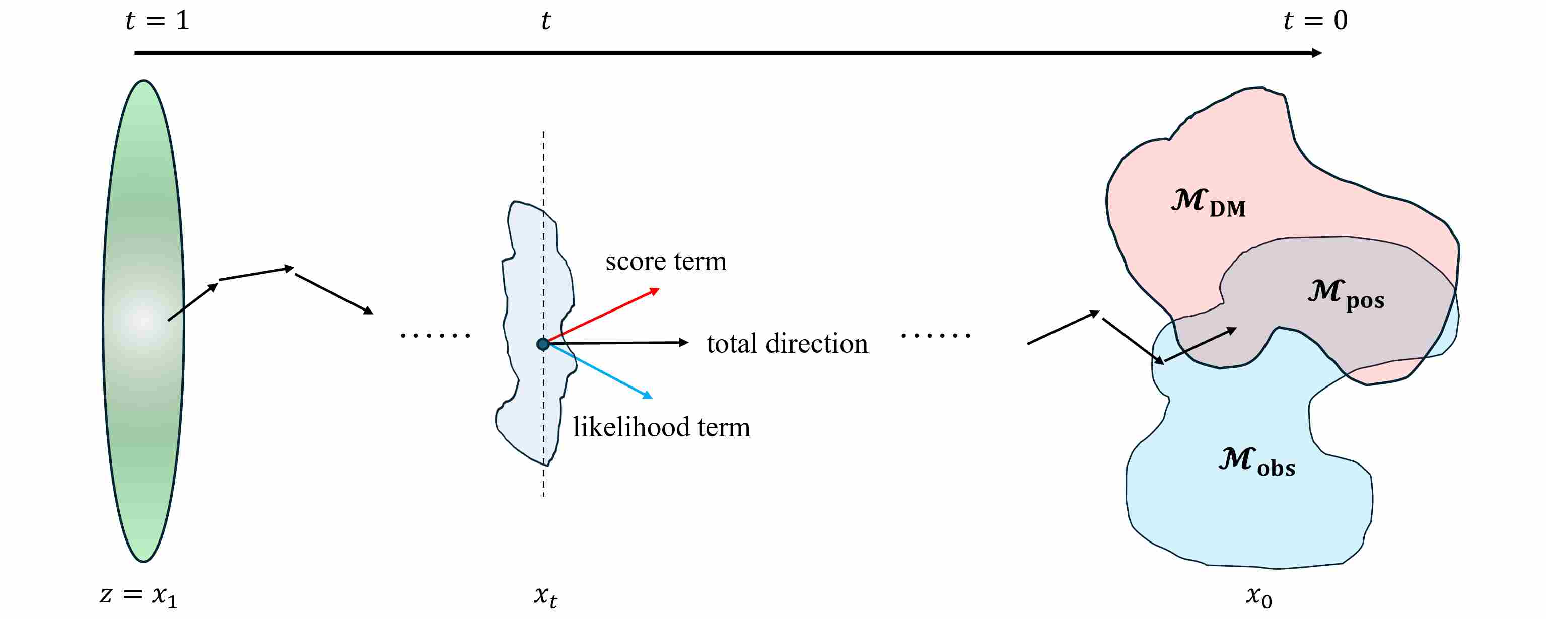
5. Posterior-Guided Sampling for Inverse Problems

In this section, we focus on posterior-guided sampling ^{20 21 22}, a paradigm for solving inverse problems from the perspective of sampling. In this paradigm, we embed the inverse problem into the reverse-time dynamics of the diffusion model by replacing the prior score with a posterior score:

and then simulate a modified reverse SDE/ODE whose stationary distribution at \(t\!=\!0\) coincides with the desired posterior \(p(\mathbf{x}_0\mid \mathbf{y})\). The following figure shows the process of posterior-guided sampling

Figure 1: Posterior-Guided Sampling for Inverse Problems

5.1 Why Inverse Problems Can Be Solved by Sampling: A Fokker–Planck View

We begin with the unconditional case. Let \(\{ \mathbf{x}_t \}_{t\in[0,T]}\) be the forward noising process of a diffusion model,

with \(\mathbf{w}_t\) a standard Wiener process and \(p_t(\mathbf{x}_t)\) the marginal density at time \(t\). The evolution of \(p_t\) is governed by the Fokker–Planck equation ^{19 20}

Score-based diffusion models rely on the fact that there exists a reverse-time SDE

whose marginals also satisfy the same Fokker–Planck equation but evolve backward in time from \(t=T\) to \(t=0\). If we start from \(\mathbf{x}_T \sim p_T \approx \mathcal{N}(0,I)\) and integrate the reverse SDE/ODE with the true score \(\nabla_{\mathbf{x}_t}\log p_t(\mathbf{x}_t)\), then the marginals of \(\mathbf{x}_t\) are exactly \(\{p_t\}_{t\in[0,T]}\), and in particular \(\mathbf{x}_0\sim p_{\text{data}}\).

Now consider an inverse problem with measurements

Conditioning on \(\mathbf{y}\) lifts to the full diffusion trajectory: we obtain a posterior process \({\mathbf{x}_t\mid \mathbf{y}}\) with marginals \(p(\mathbf{x}_t\mid \mathbf{y})\). The corresponding Fokker–Planck equation for the posterior densities is

By the same reasoning as in the unconditional case, there exists a posterior reverse SDE

such that, if we initialize at \(t = T\) with \(\mathbf{x}_T\sim p(\mathbf{x}_T\mid \mathbf{y})\) (which is typically close to the unconditional \(p_T\)), then the marginals of \(\mathbf{x}_t\) follow \({ p(\mathbf{x}_t\mid \mathbf{y}) }_{t\in[0,T]}\), and finally

This gives the fundamental justification: If we can approximate the posterior score \(\nabla_{\mathbf{x}_t}\log p(\mathbf{x}_t\mid \mathbf{y})\) and integrate the corresponding reverse-time dynamics, then sampling the inverse problem reduces to simulating a posterior-guided diffusion process whose terminal distribution at \(t\to 0\) is exactly the desired posterior \(p(\mathbf{x}_0\mid \mathbf{y})\).

In other words, inverse problems can be solved by sampling because the Fokker–Planck equation guarantees that the reverse-time SDE with the posterior score has the posterior as its stationary marginal at $t=0$. The remaining question is how to approximate this posterior score in practice.

5.2 Constructing Posterior-Guided Reverse Dynamics

By Bayes’ rule,

so the posterior score decomposes as

Diffusion training gives us a learned prior score

so the main missing piece is the likelihood score. Assuming we can approximate it (we discuss in section 5.3), the posterior-guided reverse ODE becomes

In practice, this continuous-time dynamics is discretized at a sequence of times

Return \(\mathbf{x}_0\) at the end of the trajectory as a sample from an approximate posterior over clean images.

5.3 Approximating the Likelihood Score via the Clean Space

We now address the core technical difficulty: how to approximate the likelihood score

Under the standard linear-Gaussian measurement model, the likelihood is defined in the clean space:

with gradient

However, the diffusion model operates in the noisy space \(\mathbf{x}_t\), related to \(\mathbf{x}_0\) via the forward noising process, e.g.

The noisy-space likelihood is obtained by marginalizing over \(\mathbf{x}_0\):

This integral is intractable in high dimensions, and differentiating \(\log p(\mathbf{y}\mid \mathbf{x}_t)\) w.r.t. \(\mathbf{x}_t\) would require full access to the conditional distribution \(p(\mathbf{x}_0\mid \mathbf{x}_t)\), which we do not have explicitly.

Posterior-guided methods therefore rely on a concentration assumption: for a given \((\mathbf{x}_t, t)\), the conditional distribution \(p(\mathbf{x}_0\mid \mathbf{x}_t)\) is sharply peaked around a denoised estimate

Approximating \(p(\mathbf{x}_0\mid \mathbf{x}_t)\) by a delta measure at \(\hat{\mathbf{x}}_0\) (a Laplace / delta approximation) yields

This is the key approximation, we differentiate this approximate expression w.r.t. \(\mathbf{x}_t\), we obtain

5.4 Geometric interpretation: the Jacobian as a projection onto the tangent space

Likelihood score described above is not merely algebra. The crucial insight is geometric: under standard manifold assumptions, this Jacobian behaves like a projection onto the tangent space of the data manifold.

Assume that the clean data \(\mathbf{x}_0\) lie (locally) on a smooth low-dimensional manifold \(\mathcal{M}\subset\mathbb{R}^d\), and that the denoiser \(\hat{\mathbf{x}}_0(\mathbf{x}_t,t)\) acts as a projection back to the manifold:

Intuitively, given a noisy point \(\mathbf{x}_t\) near \(\mathcal{M}\), the denoiser snaps it back to the nearest point \(\hat{\mathbf{x}}_0\in\mathcal{M}\). Now consider a small perturbation \(\delta \mathbf{x}_t\) around \(\mathbf{x}_t\). We can decompose it as

where \(T_{\hat{\mathbf{x}}_0}\mathcal{M}\) is the tangent space of the manifold at \(\hat{\mathbf{x}}_0\).

• If we move \(\mathbf{x}_t\) along the tangent direction \(\delta \mathbf{x}_{\text{tan}}\), the projected point \(\hat{\mathbf{x}}_0(\mathbf{x}_t,t)\) will move along the manifold in essentially the same direction.

• If we move \(\mathbf{x}_t\) along the normal direction \(\delta \mathbf{x}_{\text{nor}}\), the nearest point on the manifold changes very little—projection “drops” the normal component.

Linearizing this behavior, we obtain

This shows that, to first order,

i.e. the Jacobian of the denoiser “keeps” the tangent component and discards the normal component. In other words, \(J_{\hat{\mathbf{x}}_0}(\mathbf{x}_t)\) acts as a projection operator from the ambient space \(\mathbb{R}^d\) onto the tangent space \(T_{\hat{\mathbf{x}}_0}\mathcal{M}\).

Putting this back into the likelihood score expression, looking at the Eq. \ref{eq:lik} above, we can easily see that the likelihood score actually consists of two parts.

Geometrically, this means:

• First, we compute the clean-space measurement gradient:

  \[\mathbf{g}_{x_0} = \frac{1}{\sigma^2} \mathbf{A}^\top(\mathbf{y}-\mathbf{A}\hat{\mathbf{x}}_0),\]

  which tells us how to move \(\hat{\mathbf{x}}_0\) to better satisfy \(\mathbf{A}\mathbf{x}_0\approx\mathbf{y}\).

• Then, we apply \(J_{\hat{\mathbf{x}}_0}^\top\) (which behaves like a projection onto \(T_{\hat{\mathbf{x}}_0}\mathcal{M})\) to this gradient, removing its normal component and keeping only the tangent component along the data manifold.

The result is a likelihood score in noisy space that moves \(\mathbf{x}_t\) in a direction that: improves data consistency (because it originates from \(\mathbf{g}_{x_0}\)), and remains compatible with the learned data manifold (because it is projected to the tangent space).

5.5 Operator Splitting: Balancing Prior and Likelihood in Practice

Finally, we discuss a key algorithmic design pattern in posterior-guided sampling: operator splitting between prior and likelihood contributions. We can directly substitute the posterior score into Eq. \ref{eq:pgs} and use an ODE solver to sample $x_0$. However, in practice, we typically break this process down into two steps.

Instead of integrating the full posterior vector field in one monolithic update, we decompose each step into prior step and data-consistency (DC) step. Mathematically, this corresponds to splitting the posterior vector field:

and discretizing one time step as

where

This seemingly simple splitting brings several concrete benefits:

• Explicit control of the prior–likelihood trade-off. The DC step size and schedule (e.g., \(\eta_k\) as a function of \(t_k\)) directly encode how strongly we trust the measurements at different noise levels. We can use weaker DC updates at large $t$ (when \(\hat{\mathbf{x}}_0\) is unreliable) and stronger updates near $t=0$, without modifying the underlying prior sampler.

• Modularity and reuse of samplers. The prior step can be any off-the-shelf diffusion or flow-matching sampler. Adapting to a new inverse problem then only requires changing the DC step (i.e., the likelihood term), rather than redesigning a full posterior-guided integrator from scratch.

• Improved stability and interpretability. When posterior updates misbehave, splitting makes it clear which part is responsible: unstable behavior often comes from overly aggressive DC steps rather than from the prior dynamics. This separation makes it easy to clip, damp, or project only the DC update, while keeping the prior sampler untouched.

In summary, “prior step + DC step” can be viewed as a structured approximation to posterior-guided dynamics that preserves the benefits of diffusion priors, while offering fine-grained, problem-specific control over data fidelity and stability.

6. Clean Space Local-MAP optimization Paradigm

In section 5, we viewed diffusion-based inverse problem solvers as posterior-guided samplers in the noisy space \(\{\mathbf{x}_t\}_{t\in[0,T]}\): by replacing the prior score with the posterior score and sampling through the reverse SDE or PF-ODE, the final sampling result is the solution to the inverse problem.

In this chapter we turn to a complementary perspective, exemplified by Decomposed Diffusion Sampling (DDS) ²³, where the inverse problem is addressed via local optimization in the clean space \(\mathbf{x}_0\).

6.1 From Global MAP to Local Clean-Space Optimization

We consider the standard linear inverse problem

together with a diffusion prior that implicitly defines a distribution \(p(\mathbf{x}_0)\) via its forward noising process and learned reverse dynamics.

The global Bayesian target of interest is the clean-space MAP estimator

As discussed in Chapter 4, directly minimizing this objective is difficult. The local-MAP viewpoint used by DDS circumvents these obstacles via two key ideas.

(a) Denoised estimates as local prior anchors. For any noisy state \(\mathbf{x}_t\), the diffusion model provides a denoised prediction

obtained e.g. by Tweedie’s formula or an equivalent \(x_0\)-prediction head. Geometrically and probabilistically, this point can be interpreted as a local anchor on the data manifold:

• \(\hat{\mathbf{x}}_0\) lies close to the high-density region of \(p(\mathbf{x}_0)\) (the learned data manifold);

• in a neighborhood of \(\hat{\mathbf{x}}_0\), the prior can be approximated by a local Gaussian surrogate

  \[p(\mathbf{x}_0) \approx \mathcal{N}(\hat{\mathbf{x}}_0, \Sigma_t),\]

  for some positive-definite \(\Sigma_t\) that depends on \(t\).

Expanding the negative log-prior around \(\hat{\mathbf{x}}_0\) gives

which is exactly a quadratic trust-region penalty around the prior anchor.

Substituting this into the negative log-posterior yields the local surrogate posterior

If we absorb \(\Sigma_t^{-1}\) into a scalar weight \(\gamma\) (or into a diagonal preconditioner), this leads to the local MAP subproblem

Thus, each DDS update can be viewed as solving a local approximation of the global MAP problem in which the intractable prior is replaced by a tractable quadratic surrogate around \(\hat{\mathbf{x}}_0\).

(b) Iterating local surrogates is appropriate to optimizing the global posterior. Solving \ref{eq:local_map} at a single time step only gives a local improvement. However, along the diffusion trajectory:

1. The outer dynamics gradually move \(\hat{\mathbf{x}}_0(\mathbf{x}_t, t)\) along the data manifold governed by the diffusion prior.
2. At each time \(t_k\), (6.1) constructs a local surrogate of the global posterior around the current anchor \(\hat{\mathbf{x}}_0(\mathbf{x}_{t_k}, t_k)\).

3. By repeatedly updating \(\mathbf{x}_0\) via these surrogates and lifting it back to \(\mathbf{x}_{t_{k-1}}\), we obtain a sequence whose clean endpoints

   \[\mathbf{x}_0^{(K)}, \mathbf{x}_0^{(K-1)}, \dots, \mathbf{x}_0^{(0)}\]

   approximate a descent trajectory of the true negative log-posterior.

This is closely analogous to majorization–minimization / proximal point methods in classical optimization.

6.2 How Local-MAP Optimization Is Implemented

We now outline how the local-MAP paradigm is realized in practice, following the structure of DDS²³. Consider a decreasing time schedule

At each step, we perform three main operations.

Step 1 — Prior projection to the clean space. Given a noisy state \(\mathbf{x}_{t_k}\) at time \(t_k\), we first apply a pure prior step (e.g. PF-ODE, DDIM, or any high-order diffusion solver) without any data-consistency (DC) term, and then compute a denoised estimate:

This estimate can be interpreted as the local mode or mean of the conditional prior \(p(\mathbf{x}_0\mid\mathbf{x}_{t_k})\). It lives near the data manifold and serves as the anchor in the local subproblem.

Step 2 — Solve a clean-space local MAP subproblem. Next, we solve the local optimization problem

where \(\gamma_k>0\) controls the relative strength of the data term at time \(t_k\). This is a convex quadratic problem whenever \(A^\top A\) is positive semidefinite, which is the case for typical linear measurement operators. Optimization methods such as conjugate gradients (CG), which only require repeated applications of \(A\) and \(A^\top\) and thus scale to very high-dimensional imaging problems. Intuitively, the solution \(\mathbf{x}_0^{\star,(k)}\) performs a locally optimal trade-off between:

• staying close to the prior anchor \(\hat{\mathbf{x}}_0^{(k)}\) (trust-region term);
• reducing the data consistency mismatch \(\|\mathbf{y}-\mathbf{A}\mathbf{x}_0\|^2\).

Figure 2: Local Map Optimization

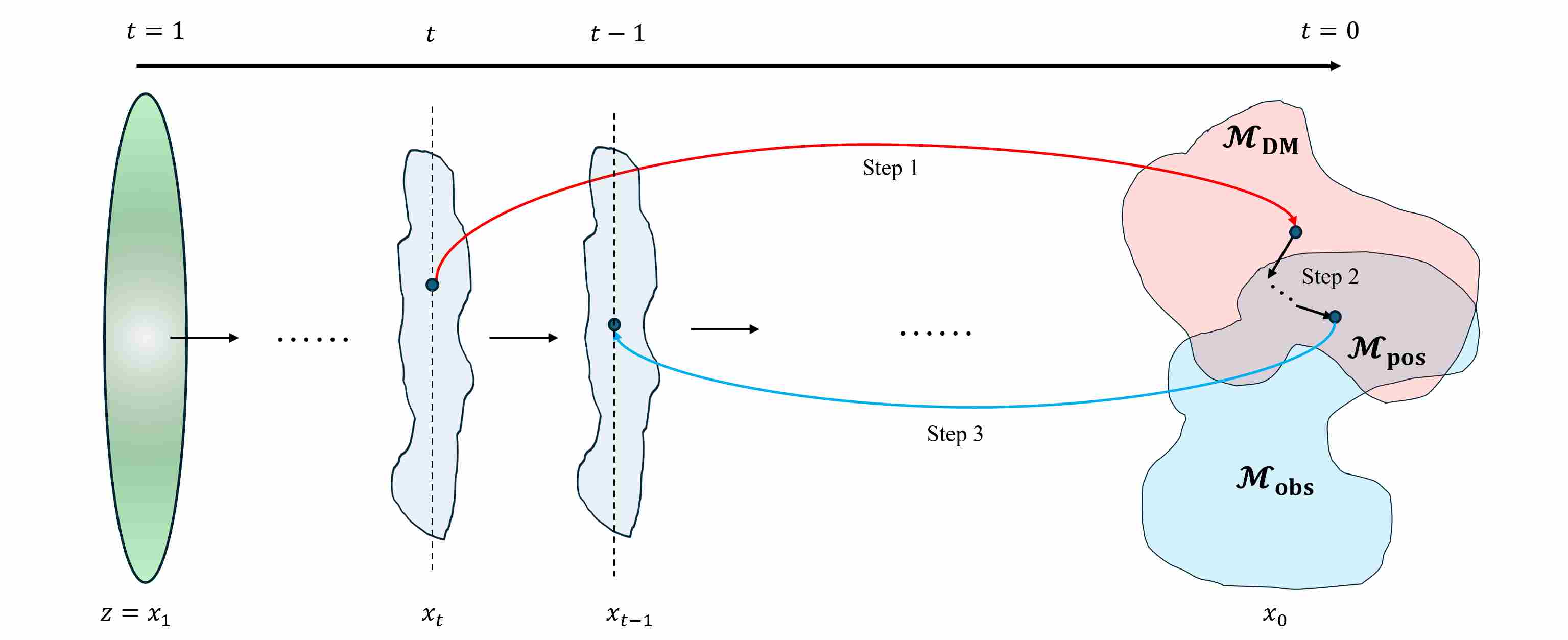
Step 3 — Re-noise to continue the diffusion trajectory. Finally, the updated clean estimate \(\mathbf{x}_0^{\star,(k)}\) is mapped back to the next noisy state \(\mathbf{x}_{t_{k-1}}\) using the forward noising kernel corresponding to the chosen diffusion parameterization (VP/VE) or its deterministic DDIM/ODE variant:

This completes one outer iteration. Starting from an initial sample \(\mathbf{x}_{t_K} \sim \mathcal{N}(\mathbf{0}, I)\), we repeat Steps 1–3 for \(k = K, K-1, \dots, 0\). The final clean estimate.

6.3 Practical Advantages of Local-MAP Optimization

Compared with posterior-guided sampling in the noisy space (Chapter 5), the local-MAP view brings a different algorithmic factorization of the same Bayesian inverse problem. Instead of injecting the likelihood directly into the reverse dynamics of $\mathbf{x}_t$, it keeps the diffusion prior as a pure generative trajectory and enforces data consistency only through clean-space optimization. This seemingly small change has several concrete consequences.

(a) Exact likelihood treatment in the space of interest. In local-MAP methods, data consistency is always enforced in the clean space:

so the likelihood term is used in its original form \(\log p(\mathbf{y}\mid\mathbf{x}_0)\), without pushing it through the denoiser \(\hat{\mathbf{x}}_0(\mathbf{x}_t,t)\) or approximating \(\nabla_{\mathbf{x}_t}\log p(\mathbf{y}\mid\mathbf{x}_t)\).

All approximation is confined to the prior side (via the quadratic surrogate around \(\hat{\mathbf{x}}_t\)), while the measurement model and its gradient remain exact. This makes each update transparently interpretable as a local MAP step for the original inverse problem.

(b) Manifold-aware updates without Jacobians. The denoised estimate $\hat{\mathbf{x}}_t$ lies close to the diffusion data manifold. The quadratic term

acts as a trust region centered at this point: the optimizer is encouraged to improve data fidelity, but discouraged from moving far away from the manifold in a single step. As a result, the update direction behaves like a tangent-space-projected likelihood gradient, yet this projection is implemented implicitly by the penalty, not via explicit Jacobian–vector products as in MCG. In practice this retains the geometric benefits of manifold-constrained optimization while avoiding the cost and instability of differentiating $\hat{\mathbf{x}}_0$ with respect to $\mathbf{x}_t$.

(c) Modular separation of prior trajectory and inverse solver. Finally, the local-MAP formulation separates the roles of the diffusion model and the inverse solver:

• the prior module provides a sequence of anchors $\hat{\mathbf{x}}_t$ and noise levels through unconditional (or weakly guided) sampling in $\mathbf{x}_t$;
• the optimization module solves, at each time step, a purely clean-space problem such as (6.1) using standard numerical linear algebra (CG, preconditioning, multi-grid, etc.).

No gradients are backpropagated through the diffusion network with respect to $\mathbf{A}$ or $\mathbf{y}$, and the clean-space solver only needs calls to $\mathbf{A}$ and $\mathbf{A}^\top$. This modularity makes it easy to swap samplers, change forward operators, or upgrade the inner optimizer without redesigning the whole algorithm, and connects diffusion-based inverse solvers to the rich toolbox of classical optimization methods.

7. Other Paradigms for Diffusion-Based Inverse Solvers

The previous two chapters detailed the two most dominant paradigms for solving inverse problems with diffusion priors: posterior-guided sampling in the noisy space and local-MAP optimization in the clean space. While these frameworks cover a large portion of modern techniques, several other powerful algorithmic families exist, each offering a unique perspective and a different set of trade-offs between computational cost, theoretical rigor, and implementation complexity.

This chapter provides a brief overview of three such alternative paradigms, highlighting their core ideas and how they differ from the methods discussed earlier.

7.1 Variational and Amortized-Inference Formulations

A first family that goes beyond “solve one inverse problem at a time” is variational inference with diffusion priors. Instead of directly computing a MAP point or running a sampler for each measurement \(\mathbf{y}\), these methods introduce a tractable, parameterized approximation \(q_\phi(\mathbf{x}_0 \mid \mathbf{y})\) of the posterior and optimize \(\phi\) by minimizing a variational divergence such as

Conceptually, this moves the computational burden from test-time to training-time:

• During training, the model learns an amortized mapping

  \[\mathbf{y} \mapsto q_\phi(\mathbf{x}_0\mid\mathbf{y}),\]

  often implemented by a neural network that outputs either a mean (for MAP-like reconstructions) or parameters of a distribution from which samples can be drawn.

• At test time, solving the inverse problem reduces to a single forward pass through the inference network, optionally followed by a small number of refinement steps (e.g., gradient descent or short posterior-guided sampling).

From the perspective of this article, such methods usually combine elements of both core paradigms:

• When the objective for (\phi) is derived from a time-discretized diffusion process, its gradient typically involves Monte Carlo estimates of a posterior score, and the training dynamics resemble a learned version of posterior-guided sampling (Chapter 5).
• When the inference network outputs a point estimate (\hat{\mathbf{x}}_0(\mathbf{y})) and is trained via a surrogate for the negative log-posterior, the learned mapping behaves like a global, amortized MAP solver in clean space, conceptually related to the local-MAP perspective of Chapter 6 but with a single shot instead of per-instance inner iterations.

Thus, variational and amortized-inference approaches do not introduce a fundamentally different objective, but rather change where and how the optimization is performed: they compress the repeated optimization/sampling over (\mathbf{x}_0) into a shared set of parameters (\phi), trading training cost and model capacity for fast test-time inference.

7.2 CSGM-type and Latent-Space Optimization

Conceptually, the latent-space optimization methods with diffusion priors are not a new paradigm. They are the diffusion-family analogue of the latent-MAP strategies already introduced in Chapter 3 for GANs and VAEs.

Briefly, the latent-space optimization is also known as CSGM (Compressed Sensing using Generative Models) ²⁴ when the forward operator $A$ corresponds to a compressive sensing matrix and \(G_\theta\) is a pretrained generator. In this subsection, we revisit the same CSGM-type idea, but instantiate the generator \(G_\theta\) with a diffusion-family prior instead of a GAN or VAE. The algorithmic template is identical:

1. Use a generative model \(G_\theta\) to parameterize the data manifold.
2. Introduce a latent variable \(\mathbf{z}\) (the “code” or “initial state”).
3. Solve the inverse problem by optimizing \(\mathbf{z}\) so that \(G_\theta(\mathbf{z})\) both matches the measurements and stays compatible with the prior.

Formally, for a known forward operator \(A\) and Gaussian noise, we again consider an objective of the form

7.2.1 Implementation: backpropagation through the sampler, not explicit Jacobians

At first sight, treating a diffusion sampler as \(G_\theta\) may seem to require computing a Jacobian for every denoising step. If we write the sampler as a composition

where each \(F_t\) maps \(\mathbf{x}_t \mapsto \mathbf{x}_{t-1}\), then mathematically

and the latent gradient

appears to involve all these Jacobians. In practice, however, we never form these Jacobians explicitly. Modern autodiff frameworks compute \(\nabla_{\mathbf{z}} L\) by a single end-to-end backward pass: internally, this backward pass performs a sequence of Jacobian–vector products for each step \(F_t\), chaining them together via the usual reverse-mode automatic differentiation, so we do not explicitly compute “one big Jacobian per step” and multiply them.

However, we do pay for each step during backpropagation, the cost of one gradient step in \(\mathbf{z}\) is roughly “one additional sampling run”, and we must also store (or recompute) intermediate activations for all steps, which can be memory intensive. This is the key efficiency difference compared to GANs/VAEs.

7.2.2 When is diffusion-based latent optimization practically useful?

Because of this scaling, latent-space optimization with diffusion priors is usually not attractive on top of a full 50–1000-step sampler. In practice, the CSGM-style latent optimization with diffusion priors is much more compelling when:

• The diffusion prior has been distilled into a single- or few-step sampler, such as LCM- or CTM-like models, or

• The prior is a consistency model that already defines a one- or two-step map \(\mathbf{x}_0 = F_\theta(\mathbf{z})\).

Methods like DMPlug ²⁵ make this approach feasible by using a significantly reduced number of sampling steps. The advent of Consistency Models ²⁶, which distill the ODE into a single-step generator, makes this paradigm much more practical, as inverting a single function call is computationally equivalent to inverting a GAN.

7.3 Asymptotically Exact Bayesian Samplers

Sections 5 and 6 focused on efficient but approximate solvers: posterior-guided sampling in noisy space and local-MAP optimization in clean space. In contrast, a third line of work aims to construct asymptotically exact Bayesian samplers, i.e., algorithms whose limiting distribution is the true posterior

where the prior \(p(\mathbf{x}_0)\) is implemented by a diffusion model. In this section we abstract two representative families:

1. Markov chain Monte Carlo (MCMC): construct a Markov chain whose stationary distribution is \(\pi(\mathbf{x}_0)\);

2. Sequential Monte Carlo (SMC): maintain a weighted particle system that tracks a sequence of intermediate distributions bridging prior and posterior.

Both paradigms are asymptotically exact in the sense that, under standard conditions, their empirical distributions converge to the true posterior as the number of iterations (MCMC) or the number of particles (SMC) tends to infinity. In practice, however, the required computational budget is often prohibitive in high-dimensional imaging problems, so these methods serve more as conceptual baselines and tools for uncertainty quantification than as default reconstruction schemes.

8. Conclusion

This post has traversed the landscape of inverse problems, charting the evolution of regularization from classical analytical priors to the modern era of deep generative models. We began by revisiting how handcrafted assumptions—such as smoothness, sparsity, and self-similarity—served as the foundational bedrock for regularizing ill-posed problems. While mathematically elegant, these explicit priors often struggle to capture the complex, high-dimensional distributions of natural signals.

The transition to deep generative models, including GANs, VAEs, and Normalizing Flows, marked a shift towards data-driven manifolds. These models allowed us to replace human-designed constraints with learned distributions, transforming inverse problems into searches over latent spaces or constrained optimizations on learned manifolds.

However, the central contribution of this exposition lies in clarifying the paradigm shift introduced by Diffusion Models. Unlike their predecessors, diffusion priors do not rely on explicit low-dimensional parameterizations. Instead, they define the data manifold implicitly through stochastic trajectories and score fields. We have provided a unified view of the two dominant strategies for harnessing these powerful priors:

1. Posterior-Guided Sampling (Noisy Space): We showed how inverse problems can be solved by modifying the reverse-time dynamics. By interpreting the Jacobian of the denoiser as a projection onto the tangent space of the data manifold, we revealed that methods like DPS and MCG are essentially performing manifold-constrained gradient descent within the generative process.
2. Local-MAP Optimization (Clean Space): Conversely, we explored methods like DDS that decouple the generative process from the measurement operator. By treating the denoiser as a provider of local “trust region” anchors, these algorithms transform the intractable global Bayesian problem into a sequence of convex, clean-space optimization steps.

Ultimately, solving a generative inverse problem is an act of balancing data fidelity (matching the measurements $\mathbf{y}$) with perceptual quality (staying on the manifold defined by $p(\mathbf{x})$). Diffusion models excel at this task not just because they generate high-quality samples, but because they allow us to break down a complex, non-convex optimization problem into a sequence of manageable, local sub-problems—whether in the noisy score domain or the clean signal domain.

As the field advances towards faster samplers (e.g., Consistency Models) and more robust posterior approximations, the boundary between “optimization” and “sampling” will continue to blur. Yet, the fundamental geometric intuition established here—of navigating a learned manifold under the guidance of physical measurements—remains the guiding principle for future research.

9. References