A “flow map” ^{1 2 3} typically denotes a neural network (or parametric model)

that maps a state at time $t$ directly to a state at a time $s < t$ (often earlier), following the underlying probability-flow ODE or other transport dynamics.

In classical diffusion and flow-matching generative frameworks, the state at time $s$ can be obationed by numerical integration: starting from $x_t$, and perform multiple ODE solver steps to reach $x_s$.

where $v$ is a vector field. We use \(\Phi_{t\to s}(x_t)=x_s\) to represent the exact solution operator.

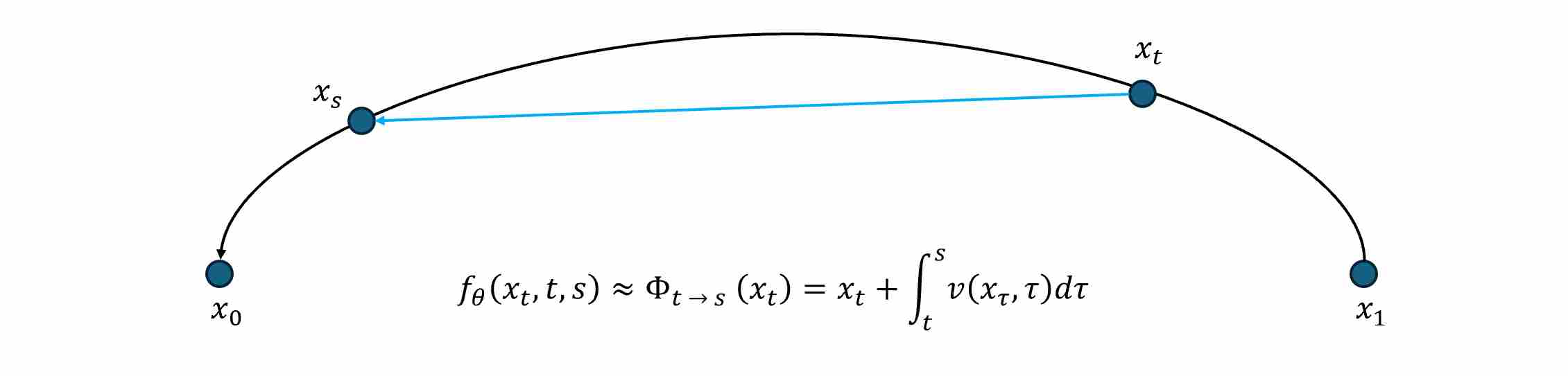
The Flow Map paradigm rethinks this process from a functional perspective. Instead of iteratively integrating a differential equation, it seeks to learn the entire solution operator of that equation, that is to say， a flow map network $f_{\theta}$ aims to approximate this operator family:

Hence, Flow Map learning transforms diffusion sampling from an integration problem into a function-approximation problem: learn the end-to-end mapping between noise levels, and then generate in one or a few evaluations.

1. Relationship Between Flow Map and Existing Model Families

The Flow Map formulation provides a unified lens through which a wide range of diffusion- and flow-based acceleration methods can be interpreted as special cases or discrete approximations.

1.1 Connection to Consistency Model (CM)

The Consistency Model ⁴ learns a neural mapping that directly transforms a partially-noised sample $x_t$ into its clean endpoint $x_0$:

This can be exactly recovered from Flow Map by setting the target time to the endpoint $s=0$:

Hence, CM is a boundary-anchored Flow Map that only learns mappings terminating at the data manifold. While CM focuses solely on consistency between the intermediate prediction $f_{\theta}(x_t,t)$ and the ground-truth $x_0$, Flow Map generalizes this to consistency between any two time instants $(t,s)$, enabling dense self-consistency supervision throughout the temporal domain.

This extension alleviates the “boundary overfitting” problem of CM and allows richer supervision that benefits both few-step and multi-step generation.

1.2 Connection to Flow Matching (FM)

The Flow Matching objective ⁵ trains a velocity field $v_\theta(x,t)$ that matches the teacher ODE:

This can be viewed as the infinitesimal limit of the Flow Map as the source and target times approach each other:

Thus,

revealing that FM emerges as the differential limit of Flow Map. Conceptually, FM learns the infinitesimal generator of the Flow Map, whereas Flow Map learns the finite-time transport operator itself.

Consequently, Flow Map can be interpreted as an integrated version of FM, capable of performing large temporal jumps without solving an ODE numerically.

1.3 Connection to MeanFlow

The MeanFlow formulation ⁶ parameterizes the flow mapping linearly with respect to the time interval:

Here (u_\theta) predicts the average velocity between $t$ and $s$:

This is precisely a re-parameterization of the Flow Map itself—MeanFlow enforces linear interpolation along the temporal interval, effectively constraining $f_{\theta}$ to obey a first-order Euler discretization.

Hence, Flow Map and MeanFlow are functionally equivalent; the only difference lies in parameterization: Flow Map directly learns the endpoint mapping $x_t\mapsto x_s$, whereas MeanFlow learns the average velocity that integrates to the same endpoint.

From a numerical perspective, Flow Map corresponds to solving the ODE with one explicit Euler step whose increment is predicted by $u_\theta$.

1.4 Connection to Consistency Trajectory Model (CTM)

The Consistency Trajectory Model (CTM) ⁷ can be viewed as the discrete-time instantiation of the Flow Map principle ¹. CTM enforces discrete trajectory consistency:

where $t_2>t_1>t_0$. This condition is a discrete approximation of the composition consistency that Flow Map satisfies exactly in the continuous limit:

Therefore, CTM can be interpreted as a time-discretized Flow Map trained on finite intervals, ensuring that two short-step predictions compose to the same endpoint as a single long-step prediction.

2. Flow Map Training: Objective and Methods

Let a pretrained teacher vector field $v_\phi(x,t)$ define the continuous probability-flow ODE

The goal of the Flow Map model is to train a neural operator

that can jump from any noise level $t$ to any target level $s$ in one step. Formally, the objective minimizes the deviation between the student flow map $f_\theta$ and the teacher flow solution:

Since the true map $\Phi_{t\to s}$ is unavailable in closed form, we approximate it using the teacher vector field and construct distillation losses that align the local behavior of $f_\theta$ with the teacher ODE.

Two complementary formulations arise, corresponding to the Eulerian and Lagrangian viewpoints of fluid dynamics.

2.1 Eulerian Map Distillation (EMD)

EMD fixes the target time $s$ and requires that the prediction at this endpoint be invariant when the starting point $(x_t,t)$ moves infinitesimally along the teacher trajectory. It enforces temporal consistency of the flow map at a fixed destination.

2.1.1 Discrete Form

For a small step:

and

the Eulerian consistency loss is

where $f_{\theta^-}$ is a stop-gradient copy (no back-prop through the reference branch). This simple MSE form avoids Jacobian–vector-product instabilities and scales well to high-dimensional images.

2.2 Lagrangian Map Distillation (LMD)

LMD fixes the starting point $(x_t,t)$ and enforces that, when the endpoint $s$ changes slightly, the flow-map prediction evolves consistently with the teacher’s instantaneous velocity. It aligns the terminal direction of the student with the teacher vector field—mirroring the Lagrangian, “follow-the-particle” viewpoint.

2.2.1 Discrete Form

For a nearby endpoint:

let \(y' = f_{\theta^-}(x_t,t,s')\) and move it through the teacher ODE one Euler step:

Then the loss is

3. References