
Accelerating Diffusion Sampling: From Multi-Step to Single-step Generation
📅 Published: | 🔄 Updated:
📘 TABLE OF CONTENTS
- Part I — Foundation and Preliminary
- 1. Introduction
- 2. Limitations of Classical Generative Models
- 3. The Rise of Diffusion Models
- 4. The Dual Origins of Diffusion Sampling
- Part II — Fast Sampling without Retraining
- Part III — Distillation for Fast Sampling
- 8. Trajectory-Based Distillation
- 9. Adversarial-Based Distillation
- 10. Distribution-Based Distillation
- 11. Score-Based Distillation
- 11.1 Unifying View: Distill the Score Residual
- 11.2 A Common Objective: Score Divergence
- 11.3 A Canonical Training Algorithm (Template)
- 11.4 Where Methods Differ
- 11.5 Score Distillation for Fast Sampling
- 11.6 Score Distillation for Guidance and Editing
- 11.7 Acceleration vs Guidance: Common Core, Different Endgame
- 12. Consistency-Based Distillation
- Part IV — Flow Matching: Looking for Straight Trajectory
- Part V — From Trajectory to Operator
- 15. References
This article systematically reviews the development history of sampling techniques in diffusion models. Starting from the two parallel technical routes of score-based models and DDPM, we explain how they achieve theoretical unification through the SDE/ODE framework. On this basis, we delve into various efficient samplers designed for solving the probability flow ODE (PF-ODE), analyzing the evolutionary motivations from the limitations of classical numerical methods to dedicated solvers such as DPM-Solver. Subsequently, the article shifts its perspective to innovations in the sampling paradigm itself, covering cutting-edge technologies such as consistency models and sampling distillation aimed at achieving single-step/few-step generation. Finally, we combine practical strategies such as hybrid sampling and guidance, conduct a comprehensive comparison of existing methods, and look forward to future research directions such as learnable samplers and hardware-aware optimizations.
Part I — Foundation and Preliminary
1. Introduction
The history of diffusion model sampling is a story of a relentless quest for an ideal balance within a challenging trilemma: Speed vs. Quality vs. Diversity.
Speed (Computational Cost): The pioneering DDPM (Denoising Diffusion Probabilistic Models) demonstrated remarkable generation quality but required thousands of sequential function evaluations (NFEs) to produce a single sample. This computational burden was a significant barrier to practical, real-time applications and iterative creative workflows. Consequently, the primary driver for a vast body of research has been the aggressive reduction of these sampling steps.
Quality (Fidelity): A faster sampler is useless if it compromises the model’s generative prowess. The goal is to reduce steps while preserving, or even enhancing, the fidelity of the output. Many methods grapple with issues like error accumulation, which can lead to blurry or artifact-laden results, especially at very low step counts. High-quality sampling means faithfully following the path dictated by the learned model.
Diversity & Stability: Sampling can be either stochastic (introducing randomness at each step) or deterministic (following a fixed path for a given initial noise). Stochastic samplers can generate a wider variety of outputs from the same starting point, while deterministic ones offer reproducibility. The choice between them is application-dependent, and the stability of the numerical methods used, especially for high-order solvers, is a critical area of research.
This perpetual negotiation between speed, quality, and diversity has fueled a Cambrian explosion of innovative sampling algorithms, each attempting to push the Pareto frontier of what is possible.
2. Classical Generative Models
The essence of any generative model is to build a distribution $p_{\theta}(x)$ to approximate the true data distribution $p_{\text{data}}(x)$, that is,
\[p_{\theta}(x) \approx p_{\text{data}}(x)\]Once we can evaluate or sample from $p_{\theta}(x)$, we can synthesize new, realistic data.
However, modeling high-dimensional probability densities is notoriously difficult for several intertwined reasons:
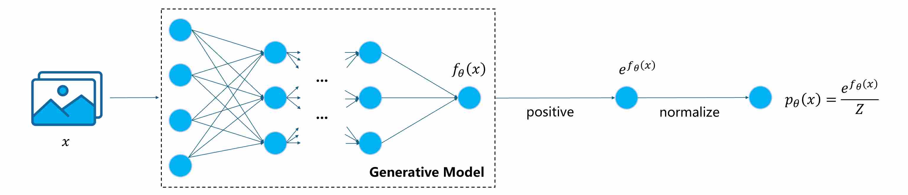
Intractable Normalization Constant. Many distributions can be expressed as
\[p_{\theta}(x)=\frac{1}{Z}\,\exp (f_{\theta}(x))\]where
\[Z=\int \exp (f_{\theta}(x))dx\]is the partition function. Computing $Z$ in high-dimensional space is intractable, making likelihood evaluation and gradient computation (with respect to $\theta$, not $x$) expensive.
Curse of Dimensionality. Real-world data (images, audio, text) lies near intricate low-dimensional manifolds within vast ambient spaces. Directly fitting a normalized density over the full space is inefficient and unstable.
Difficult Likelihood Optimization. To solve $p_{\theta}$, the most common strategy is to optimize $\log p_{\theta}(x)$ (Maximum likelihood estimation). However, maximizing $\log p_{\theta}(x)$ requires differentiating through complex transformations or Jacobian determinants—tractable only for carefully designed, such as flow models.
Although directly estimating the full data density is nearly impossible in high-dimensional space, different classes of generative models have developed specialized mechanisms to avoid or bypass the core obstacles outlined above.
Variational Autoencoders (VAEs): Approximating the Density via Latent Variables. VAEs sidestep the intractable normalization constant by introducing a latent variable $z$ and decomposing the joint distribution as
\[p_\theta(x,z)=p_\theta(x \mid z) \cdot p(z),\]Instead of maximizing $\log p_\theta(x)$ directly, the VAE introduces an approximate posterior $q_\phi(z\mid x)$ and applies Jensen’s inequality:
\[\mathcal L_{\text{MLE}} = \log p_\theta(x) \ge \underbrace{ \mathbb E_{q_\phi(z \mid x)}[\log p_\theta(x \mid z)] - \mathrm{KL}(q_\phi(z \mid x) \mid p(z))}_{\mathcal L_{\text{VLB}}}.\]Optimizing $\mathcal L_{\text{MLE}}$ requires to compute the gradient of $Z$, which is usually intractable. However, $\mathcal L_{\text{VLB}}$ contains only terms that are individually normalized and easy to compute:
- $p(z)$ is a simple prior, typically $\mathcal N(0,I)$.
$q_\phi(z \mid x)$ is an approximate posterior, which is chosen from a tractable family, e.g.
\[q_\phi(z\mid x) = \mathcal{N}(z; \mu_\phi(x), \mathrm{diag}(\sigma_\phi^2(x))).\]Its log-density is explicitly computable and differentiable with respect to $\phi$.
$\log p_\theta(x \mid z)$ is conditional likelihood, which is typically Gaussian or Bernoulli. Since the reconstruction loss is simply the negative log-likelihood of the assumed data distribution given the latent variable. the choice of conditional likelihood determines the form of the reconstructed loss function.
Conditional Likelihood $p_\theta(x \mid z)$ Reconstruction Loss $\mathcal{N}(x; \mu_\theta(z), \sigma^2 I)$ Mean Squared Error (MSE) $\mathrm{Bernoulli}(x; \pi_\theta(z))$ Binary Cross Entropy (BCE) $\mathrm{Categorical}(x; \pi_\theta(z))$ Cross Entropy $\mathrm{Laplace}(x; \mu_\theta(z), b)$ L1 Loss
Every term in the ELBO depends only on distributions that we define ourselves with explicit normalization constants, this turns an intractable integral into a differentiable objective. Sampling becomes straightforward: draw $z\,\sim\,p(z)$ and decode $x\,\sim\,p_\theta(x \mid z)$. The cost is blurriness in samples—an inevitable consequence of the Gaussian decoder and variational approximation.
Normalizing Flows: Enforcing Exact Likelihood via Invertible Transformations. Flow-based models make the density tractable by designing the generative process as a sequence of invertible mappings:
\[x = f_\theta(z),\qquad z\,\sim\,p(z).\]The change-of-variables formula yields an explicit, exact log-likelihood:
\[\log p_\theta(x)=\log p(z)-\log|\det J_{f_\theta}(z)|.\]Thus, both density evaluation and sampling are efficient and exact. However, this convenience comes with architectural constraints: each transformation must be bijective with a Jacobian determinant that is computationally cheap to compute. To maintain this property, Flow models (e.g., RealNVP, Glow) restrict the network’s expressiveness compared with unconstrained architectures.
Generative Adversarial Networks (GANs): Learning without a Normalized Density. GANs abandon likelihoods altogether. A generator $G_\theta(z)$ learns to produce samples whose distribution matches the data via an adversarial discriminator $D_\phi(x)$:
\[\min_G\max_D ; \mathbb E_{x\sim p_{\text{data}}}\,[\log D(x)] +\mathbb E_{z\sim p(z)}\,[\log(1-D(G(z)))].\]This implicit likelihood approach avoids computing $Z$, $\log p(x)$, or any Jacobian. Sampling is trivial: feed a random latent $z$ through the generator. Yet, the absence of an explicit density leads to instability and mode collapse—the model may learn to generate only a subset of modes of the true distribution.
Energy-Based Models (EBMs): Modeling Unnormalized Densities with MCMC Sampling. EBMs keep the simplest formulation of density—an unnormalized energy function $U_\theta(x)$—but delegate sampling to iterative stochastic processes like Langevin dynamics or Contrastive Divergence. The model defines:
\[p_\theta(x)=\frac{1}{Z_\theta}\exp(-U_\theta(x)).\]Because $Z_\theta$ is intractable, training relies on estimating gradients using samples from the model distribution, obtained via slow MCMC chains. This approach retains full modeling flexibility but sacrifices sampling speed and stability.
3. The Rise of Diffusion Models
Despite their conceptual elegance and individual successes, the classical families of generative models share a common limitation: they struggle to simultaneously ensure expressivity, stability, and tractable likelihoods.
VAEs approximate densities but pay the price of blurry reconstructions due to their variational relaxation.
Flow models achieve exact likelihoods, yet the requirement of invertible, volume-preserving mappings imposes severe architectural rigidity.
GANs generate sharp but unstable samples, suffering from mode collapse and non-convergent adversarial dynamics.
EBMs enjoy the most general formulation but depend on inefficient MCMC sampling and are notoriously difficult to train at scale.
These obstacles reveal a deeper dilemma: a good generative model must learn both an expressive data distribution and an efficient way to sample from it, but existing paradigms could rarely achieve both at once.
It was precisely this tension—between tractable density estimation and efficient, stable sampling—that motivated the birth of diffusion-based generative modeling. Diffusion models approach generation from an entirely different angle: rather than directly parameterizing a complex distribution, they construct it through a gradual denoising process, transforming simple noise into structured data via a sequence of stochastic or deterministic dynamics. In doing so, diffusion models inherit the statistical soundness of energy-based methods, the stability of likelihood-based training, and the flexibility of implicit generation—thereby overcoming the long-standing trade-offs that constrained previous approaches.
4. The Dual Origins of Diffusion Sampling
Before diffusion models became a unified SDE framework, two independent lines of thought evolved in parallel: One sought to model the gradient of data density in continuous space; the other built an explicit discrete Markov chain that learned to denoise. Both added noise, both removed it—yet for profoundly different reasons.
4.1 The Continuous-State Perspective: Score-Based Generative Models
The first paradigm was rooted in a fundamental question: if we had a function that could always point us toward regions of higher data probability, could we generate data by simply “climbing the probability hill”?
4.1.1 A Radical Shift — Learning the Gradient of data density
Directly modeling $p(x)$ is both theoretically and practically challenging, traditional generative models bypass these challenges through approximation or network structure constraints, but this also limits the model’s performance. One idea is that we do not learn the probability density, but instead learn the gradient of the probability density (also known as score function).
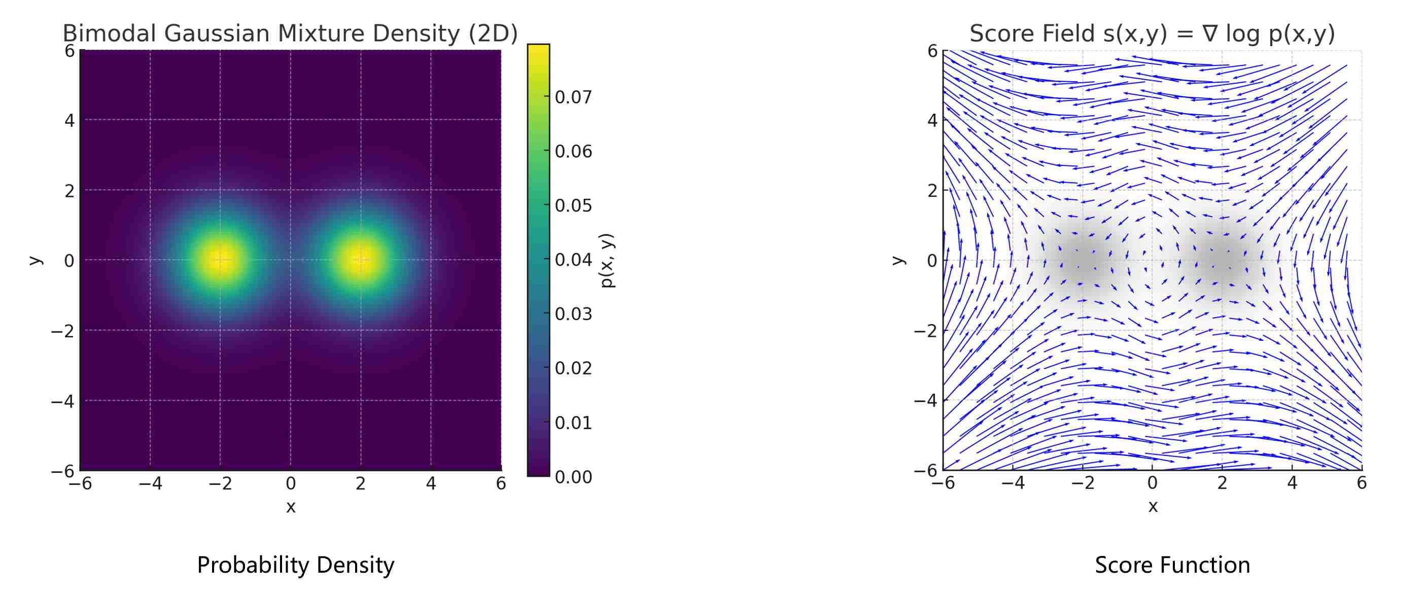
The score function, defined as
\[s(x)=\nabla_x\log p(x)\]As shown in the following figure, score function is a vector field which points toward regions of higher data probability. Learning this vector field—rather than the full density—offers two decisive advantages.
Independence from the Normalization Constant. Taking the gradient of $\log p(x)$ removes the partition function:
\[\nabla_x\log p(x) =\nabla_x\log \exp{(f_{\theta}(x))}-\nabla_x\log Z =\nabla_x\log f_{\theta}(x),\]because $Z$ is constant w.r.t. $x$. Thus, we can learn meaningful gradients without ever computing $Z$.
Direction Instead of Magnitude. The score tells us which direction in data space increases probability density the fastest. It defines a probability flow that guides samples toward high-density regions—akin to an energy-based model whose energy is \(U(x)=-\log p(x)\).
The most important one, is that the probability density and the score provide almost the same useful information, that’s because the score function and the probability density function can be converted between each other: Given the probability density, we can obtain the score by taking the derivative; conversely, given a score, we can recover the probability density by computing integrals.
4.1.2 Score Matching Generative Model
At the heart of this approach lies a powerful mathematical object: the score function, defined as the gradient of the log-probability density of the data, $\nabla_x \log p_{\text{data}}(x)$. Intuitively, the score at any point $x$ is a vector that points in the direction of the steepest ascent in data density. To calculate the score function of any input, we train a neural network $s_{\theta}(x)$ (score model) to learn the score
\[s_{\theta}(x) \approx \nabla_x \log p_{\text{data}}(x)\label{eq:1}\]The loss function is to minimize the Fisher divergence between the true data distribution and the model predicted output:
\[\mathcal{L}(\theta) = \mathbb{E}_{x \sim p_{\text{data}}}\left[ \big\|\,s_{\theta}(x) - \nabla_x \log p_{\text{data}}(x)\,\big\|_2^2 \right]\label{eq:2}\]The challenge, however, is that we do not know the true data distribution $p_{\text{data}}(x)$. This is where Score Matching comes in 1. Hyvärinen showed that via integration by parts (under suitable boundary conditions), the objective (equation \ref{eq:2}) can be rewritten in a form only involving the model’s parameters:
\[\begin{align} \mathcal{L}_{\text{SM}}(\theta) & = \mathbb{E}_{x \sim p_{\text{data}}} \left[ \frac{1}{2} \| s_\theta(x) \|^2 + \nabla_x \cdot s_\theta(x) \right] \\[10pt] & \approx \frac{1}{N}\sum_{i=1}^{N} \left[ \frac{1}{2} \| s_\theta(x_i) \|^2 + \nabla_x \cdot s_\theta(x_i) \right] \end{align}\]where $\nabla_x \cdot s_\theta(x) = {\text{trace}(\nabla_x s_\theta(x))}$ is the divergence of the score field. However, SM is not scalable especially for high-dimension data points, because the second term is the jacobin of score model.
For this purpose, Vincent introduced denoising score matching (DSM) 2 , by adding Gaussian noise to the real data $x$, the score model becomes predicting the score field of noised data $\tilde{x} = x + \sigma$.
\[s_{\theta}(\tilde{x}, \sigma) \approx \nabla_{\tilde{x}} \log p_{\sigma}(\tilde{x})\label{eq:5}\]where $p_{\sigma}$ is the data distribution convolved with Gaussian noise of scale $\sigma$, it is easy to verify that predicting $\nabla_{\tilde x} \log p_{\sigma}(\tilde x)$ is equivalent to predict $\nabla_{\tilde{x}} \log p_{\sigma}(\tilde{x} \mid x)$.
\[\begin{align} & \mathbb{E}_{\tilde{x} \sim p_{\sigma}(\tilde{x})}\left[\big\|\,s_{\theta}(\tilde{x}, \sigma) - \nabla_{\tilde x} \log p_{\sigma}(\tilde x)\,\big\|_2^2\right]\label{eq:6} \\[10pt] = \quad & \mathbb{E}_{x \sim p_{\text{data}}(x)}\mathbb{E}_{\tilde{x} \sim p_{\sigma}(\tilde{x} \mid x)}\left[\big\|\,s_{\theta}(\tilde{x}, \sigma) - \nabla_{\tilde{x}} \log p_{\sigma}(\tilde{x} \mid x)\,\big\|_2^2\right] + \text{const}\label{eq:7} \end{align}\]When $\sigma$ is small enough, $p_{\text{data}}(x) \approx p_\sigma(\tilde x)$. Optimizing Formula \ref{eq:7} does not require knowing the true data distribution, while also avoiding the computation of the complex Jacobian determinant.
\[\begin{align} \nabla_{\tilde{x}} \log p_{\sigma}(\tilde{x} \mid x) & = \nabla_{\tilde{x}} \log \frac{1}{\sqrt{2\pi}\sigma} {\exp}\left( -\frac{(\tilde{x}-x)^2}{2\sigma^2}\right) = -\frac{(\tilde{x}-x)}{\sigma^2} \end{align}\]4.1.3 NCSN and Annealed Langevin Dynamics
The first major practical realization of this idea was the Noise-Conditional Score Network (NCSN) 3. However, the authors found that the generated samples by solving \ref{eq:7} with a single small $ \sigma $ are of poor quality, the core issue is that real-world data often lies on a complex, low-dimensional manifold (high-density areas), in the vast empty spaces between data points, the score is ill-defined and difficult to estimate (low-density areas), so low-density regions are underrepresented, leading to poor generalization by the network in those areas. Their solution was ingenious: perturb the data with Gaussian noise of varying magnitudes $\sigma$ ($ \sigma_1 > \sigma_2 > \dots > \sigma_K > 0 $).
Large $ \sigma_i $: The distribution is highly smoothed, covering the global space with small, stable scores in low-density areas (easier to learn).
Small $ \sigma_i $: Focuses on local refinement, closer to $ p_{\text{data}} $.
The loss function now can be rewritten as:
\[\mathcal{L}(\theta) = \mathbb{E}_{\sigma \sim \mathcal{D}}\mathbb{E}_{x \sim p_{\text data}(x)}\mathbb{E}_{\tilde{x} \sim p_{\sigma}(\tilde{x} \mid x)}\left[\big\|\,s_{\theta}(\tilde{x}, \sigma) - \nabla_{\tilde{x}} \log p_{\sigma}(\tilde{x} \mid x)\,\big\|_2^2\right]\label{eq:8}\]With $\lambda{(\sigma)}$ balancing gradients across noise scales and $\mathcal{D}$ is a distribution over $\sigma$. To generate a sample, NCSN employed Annealed Langevin Dynamics (ALD) 3. LD 4 5 treats sampling as stochastic gradient ascent on log-density with Gaussian noise injected to guarantees to converge to the target distribution. ALD is an iterative sampling process:
Start with a sample drawn from pure noise, corresponding to a very high noise level $\sigma_{\text large}$.
Iteratively update the sample using the Langevin dynamics equation:
\[x_{i+1} \leftarrow x_i + \alpha s_{\theta}(x_i, \sigma_i) + \sqrt{2\alpha}z_i\]where $\alpha$ is a step size and $z_i$ is fresh Gaussian noise. This update consists of a “climb” along the score-gradient and a small injection of noise to encourage exploration.
Gradually decrease (or “anneal”) the noise level $\sigma_i$ from large to small. This process is analogous to starting with a blurry, high-level structure and progressively refining it with finer details until a clean sample emerges.
4.1.4 Historical Limitations and Enduring Legacy
The NCSN approach was groundbreaking, but it had its limitations. The Langevin sampling process was inherently stochastic due to the injected noise $z$ and slow, requiring many small steps to ensure stability and quality. The annealing schedule itself was often heuristic.
However, its legacy is profound. NCSN established the score function as a fundamental quantity for generative modeling and introduced the critical technique of conditioning on noise levels. It provided the continuous-space intuition that would become indispensable for later theoretical breakthroughs.
4.2 The Discrete-Time Perspective: Denoising Diffusion Probabilistic Models
Running parallel to the score-based work, a second paradigm emerged, built upon the more structured and mathematically elegant framework of Markov chains.
4.2.1 The Core Idea: An Elegant Markov Chain
Independently, Ho et al. 6 proposed a probabilistic approach that traded continuous dynamics for a discrete, analytically tractable Markov chain. Instead of estimating scores directly, DDPM proposed a fixed, two-part process.
Forward (Diffusion) Process: Start with a clean data sample $x_0$. Gradually add a small amount of Gaussian noise at each discrete timestep $t$ over a large number of steps $T$ (typically 1000). This defines a Markov chain $x_0, x_1, \dots, x_T$ where $x_T$ is almost indistinguishable from pure Gaussian noise. This forward process, $q(x_t \mid x_{t-1})$, is fixed and requires no learning.
\[q(x_t \mid x_{t-1}) = \mathcal{N}(x_t;\,\sqrt{\alpha_t}x_{t-1}, (1-\alpha_t)I)\]Reverse (Denoising) Process: Given a noisy sample $x_t$, how do we predict the slightly less noisy $x_{t-1}$? The goal is to learn a reverse model $p_{\theta}(x_{t-1} \mid x_t)$ to inverts this chain.
4.2.2 Forward Diffusion and Reverse Denoising
According to previous post, the solution of DDPM aims to maximize the log-likelihood of $p_{\text data}(x_0)$, which can be reduced to maximizing the variational lower bound, and maximizing the variational lower bound can further be derived as minimizing the KL divergence between $p_{\theta}(x_{t-1} \mid x_t)$ and $q(x_{t-1} \mid x_t, x_0)$.
\[\mathcal{L}_\text{ELBO} = \mathbb{E}_q \left[ \log p_\theta(x_0 \mid x_1) - \log \frac{q(x_{T} \mid x_0)}{p_\theta(x_{T})} - \sum_{t=2}^T \log \frac{q(x_{t-1} \mid x_t, x_0)}{p_\theta(x_{t-1} \mid x_t)} \right]\]The true posterior $q(x_{t-1} \mid x_t, x_0)$ can be computed using Bayes’ rule and the Markov property of the forward chain:
\[q(x_{t-1} \mid x_t, x_0) = \frac{q(x_t \mid x_{t-1}) q(x_{t-1} \mid x_0)}{q(x_t \mid x_0)}\]Since all three terms in the right sides are Gaussian distribution, the posterior $ q(x_{t-1} \mid x_t, x_0) $ is also Gaussian:
\[q(x_{t-1} \mid x_t, x_0) = \mathcal{N}\left( x_{t-1}; \tilde{\mu}_t(x_t, x_0), \tilde{\beta}_t I \right)\]with mean and and variance:
\[\tilde{\mu}_t(x_t, x_0) = \frac{1}{\sqrt{\alpha_t}} \left( x_t - \frac{\beta_t}{\sqrt{1 - \bar{\alpha}_t}} \epsilon \right) \quad , \quad \tilde{\beta}_t = \frac{(1 - \bar{\alpha}_{t-1}) \beta_t}{1 - \bar{\alpha}_t}\label{eq:14}\]Since our goal is to approximate distribution $ p_{\theta}(x_{t-1} \mid x_t) $ using distribution $q(x_{t-1} \mid x_t, x_0)$, this means that our reverse denoising process must also follow a Gaussian distribution, with the same mean and variance. Because the added noise in the reverse process is unknown, the training objective of DDPM is to predict this noise. We use $\epsilon_{\theta}(x_t, t)$ to represent the predicted noise output, substituting $ \epsilon $ with the noise predicted $\epsilon_{\theta}(x_t, t)$:
\[p_{\theta}(x_{t-1} \mid x_t) = \mathcal{N}\left( x_{t-1}; {\mu}_{\theta}(x_t, x_0), {\beta}_{\theta} I \right)\]where:
\[{\mu}_{\theta}(x_t, x_0) = \frac{1}{\sqrt{\alpha_t}} \left( x_t - \frac{\beta_t}{\sqrt{1 - \bar{\alpha}_t}} \epsilon_\theta(x_t, t) \right) \ \ , \ \ {\beta}_{\theta}=\tilde{\beta}_t = \frac{(1 - \bar{\alpha}_{t-1}) \beta_t}{1 - \bar{\alpha}_t}\]Sampling is the direct inverse of the forward process. One starts with pure noise $x_T \sim \mathcal{N}(0, I)$ and iteratively applies the learned reverse step for $ t = T, T-1, \dots, 1$, using the noise prediction $\epsilon_{\theta}(x_t, t)$ at each step to denoise the sample until a clean $x_0$ is obtained.
\[x_{t-1} = \frac{1}{\sqrt{\alpha_t}} \left( x_t - \frac{\beta_t}{\sqrt{1 - \bar{\alpha}_t}} \epsilon_\theta(x_t, t) \right) + \sqrt{\frac{(1 - \bar{\alpha}_{t-1}) \beta_t}{1 - \bar{\alpha}_t}} \epsilon\]4.2.3 Theoretical Elegance and Practical Bottleneck
DDPMs offered a strong theoretical foundation, stable training, and state-of-the-art sample quality. However, this came at a steep price: the curse of a thousand steps. The model’s theoretical underpinnings relied on the Markovian assumption and small step sizes, forcing the sampling process to be painstakingly slow and computationally expensive.
4.3 The Initial Convergence: Tying the Two Worlds Together
For a time, these two paradigms—one estimating a continuous gradient field, the other reversing a discrete noise schedule—seemed distinct. Yet, a profound and simple connection lay just beneath the surface. It was shown that the two seemingly different objectives were, in fact, two sides of the same coin.
The score function $s(x_t, t)$ at a given noise level is directly proportional to the optimal noise prediction $\epsilon(x_t, t)$:
\[s_{\theta}(x_t, t) = \nabla_{x_t} \log p(x_t) = -\frac{\epsilon_{\theta}(x_t, t)} { \sigma_t}\]where $\sigma_t$ is the standard deviation of the noise at time $t$.
This equivalence is beautiful. Predicting the noise is mathematically equivalent to estimating the score. The score-based view provides the physical intuition of climbing a probability landscape, while the DDPM view provides a stable training objective and a concrete, discrete-time mechanism.
With this link established, the two parallel streams began to merge into a single, powerful river. This convergence set the stage for the next major leap: breaking free from the rigid, one-step-at-a-time sampling of DDPM, and ultimately, the development of a unified SDE/ODE theory that could explain and improve upon both.
Part II — Fast Sampling without Retraining
Inference-time acceleration (training-free) treats a pretrained diffusion/score model as a fixed oracle and speeds up generation solely by changing the sampler—the time discretization, update rule, and numerical integration strategy—without modifying parameters or re-running training. Under this paradigm, we keep the same network evaluations \(f_\theta(x_t, t, c)\) but reduce the number of required evaluations (NFE) and improve stability by exploiting better discretizations (e.g., deterministic DDIM-style updates), multistep “pseudo-numerical” schemes (e.g., PNDM/PLMS), and higher-order ODE/SDE solvers tailored to diffusion dynamics (e.g., DEIS, DPM-Solver(++), UniPC).
Conceptually, these methods replace a long sequence of small Euler-like steps with fewer, more accurate steps by injecting local polynomial/exponential approximations, error-correcting history terms, or probability-flow–consistent updates. As a result, they offer a plug-and-play speed–quality trade-off: the model and training pipeline remain unchanged, and faster sampling is achieved purely through improved inference-time computation.
5. Breaking the Markovian Chain with DDIM
The stunning quality of DDPMs came at a steep price: the rigid, step-by-step Markovian chain. This constraint, while theoretically elegant, was a practical nightmare, demanding a thousand or more sequential model evaluations for a single image. The field desperately needed a way to accelerate this process without a catastrophic loss in quality. The answer came in the form of Denoising Diffusion Implicit Models (DDIM) 7, a clever reformulation that fundamentally altered the generation process.
5.1 From Stochastic Denoising to Deterministic Prediction
The core limitation of the DDPM sampler lies in its definition of the reverse process, which models $p_{\theta}(x_{t-1} \mid x_t)$. This conditional probability is what creates the strict, one-step-at-a-time dependency.
The DDIM paper posed a brilliant question: what if we don’t try to predict $x_{t-1}$ directly? What if, instead, we use our noise-prediction network $\epsilon_{\theta}(x_t, t)$ to make a direct guess at the final, clean image $x_0$? This is surprisingly straightforward. Given $x_t$ and the predicted noise $\epsilon_{\theta}(x_t, t)$, we can rearrange the forward process formula to solve for an estimated $x_0$, which we’ll call $\hat{x}_0$:
\[\hat{x}_0 = \frac{(x_t - \sqrt{1 - \bar{\alpha}_t} \, \epsilon_{\theta}(x_t, t))}{\sqrt{\bar{\alpha}_t}}\]This single equation is the conceptual heart of DDIM. By first estimating the final destination $x_0$, we are no longer bound by the previous step. We have a “map” that points from our current noisy location $x_t$ directly to the origin of the trajectory. This frees us from the Markovian assumption and opens the door to a much more flexible generation process.
5.2 The Freedom to Jump: Non-Markovian Skip-Step Sampling
With an estimate of pred \(\hat{x}_0\) in hand, DDIM constructs the next sample $x_{t-1}$ in a completely different way. It essentially says: “Let’s construct $x_{t-1}$ as a weighted average of three components”:
The “Clean Image” Component: The estimated final image predicted $\hat x_0$, pointing towards the data manifold.
The “Noise Direction” Component: The direction pointing from the clean image $x_0$ back to the current noisy sample $x_t$, represented by $\epsilon_{\theta}(x_t, t)$.
A Controllable Noise Component: An optional injection of fresh random noise.
The DDIM update equation is as follows:
\[x_{t-1} = \sqrt{\bar \alpha_{t-1}}\,{\hat x_0} + \sqrt{1-\bar \alpha_{t-1}-\sigma_t^2}\, \epsilon_{\theta}(x_t, t) + \sigma_t \, z_t\label{eq:20}\]Here, \(z_t\) is random noise, and $\sigma_t$ is a new hyperparameter that controls the amount of stochasticity. $\sigma_t = \eta \tilde{\beta}_t$, where $\tilde{\beta}_t$ is defined in DDPM (Equation \ref{eq:14})
This formulation \ref{eq:20} is non-Markovian because the calculation of $x_{t-1}$ explicitly depends on predicted $x_0$, which is an estimate of the trajectory’s origin, not just the immediately preceding state $x_t$. Because this process is no longer Markovian, the “previous” step doesn’t have to be $t-1$. We can choose an arbitrary subsequence of timesteps from the original $1, \dots, T$, for example, $1000, 980, 960, …, 20, 0$. Instead of taking 1000 small steps, we can now take 50 large jumps. At each jump from $t$ to a much earlier $s < t$, the model predicts $x_0$ and then uses the DDIM update rule to deterministically interpolate the correct point $x_s$ on the trajectory. This “skip-step” capability was a game-changer. It allowed users to drastically reduce the number of function evaluations (NFEs) from 1000 down to 50, 20, or even fewer, providing a massive speedup with only a minor degradation in image quality.
Formula \ref{eq:20} also reveals an important theory: for any $x_{t-1}$, the marginal probability density obtained through DDIM sampling is consistent with the marginal probability density of DDPM.
\[q(x_{t-1} \mid x_0 ) = \mathcal{N}(x_{t-1}; \sqrt{\bar{\alpha}_{t-1}} {x_0}, (1-\bar{\alpha}_{t-1})I)\]This is why DDIM can take large jumps and still produce high-quality images using a model trained for the one-step DDPM process.
5.3 The $\eta$ Parameter: A Dial for Randomness
DDIM introduced another powerful feature: a parameter denoted as $\eta$ that explicitly controls the stochasticity of the sampling process.
$\eta = 0$: (Deterministic DDIM): When $\eta = 0$, the random noise term in the update rule is eliminated. For a given initial noise $x_T$, the sampling process will always produce the exact same final image
x_0. This is the “implicit” in DDIM’s name, as it defines a deterministic generative process. This property is incredibly useful for tasks that require reproducibility or image manipulation (like SDEdit), as the generation path is fixed.$\eta = 1$ (Stochastic DDIM): When $\eta = 1$, DDIM adds a specific amount of stochastic noise at each step. It was shown that this choice makes the marginal distributions $p(x_t)$ match those of the original DDPM sampler. It behaves much like DDPM, offering greater sample diversity at the cost of reproducibility.
$0 < \eta < 1$ (Hybrid Sampling): Values between 0 and 1 provide a smooth interpolation between a purely deterministic path and a fully stochastic one, giving practitioners a convenient “dial” to trade off between diversity and consistency.
5.4 Bridging to a Deeper Theory: The Lingering Question
DDIM was a massive practical leap forward. It provided the speed that was desperately needed and introduced the fascinating concept of a deterministic generative path. However, its derivation, while mathematically sound, was rooted in the discrete-time formulation of DDPM. The deterministic path ($\eta=0$) worked exceptionally well, but it raised a profound theoretical question:
What is this deterministic path? If a continuous process underlies generation, can we describe this path more fundamentally?
The success of deterministic DDIM strongly hinted that the stochasticity of Langevin Dynamics and DDPM sampling might not be strictly necessary. It suggested the existence of a more fundamental, deterministic flow from noise to data. Explaining the origin and nature of this flow was the next great challenge.
This question sets the stage for our next chapter, where we will discover the grand, unifying framework of Stochastic and Ordinary Differential Equations (SDEs/ODEs), which not only provides the definitive answer but also reveals that Score-Based Models and DDPMs were two sides of the same mathematical coin all along.
6. The Unifying Framework of SDEs and ODEs
The insight behind DDIM—that sampling can follow a deterministic path derived from a learned vector field—opens the door to a more general formulation: diffusion models can be expressed as continuous-time stochastic or deterministic processes. In this chapter, we formalize that insight by introducing the Stochastic Differential Equation (SDE) and the equivalent Probability Flow Ordinary Differential Equation (ODE) perspectives. This unified view provides the theoretical bedrock for nearly all subsequent developments in diffusion sampling, including adaptive solvers, distillation, and consistency models.
6.1 From Discrete Steps to Continuous Time
The core insight is to re-imagine the diffusion process not as $T$ discrete steps, but as a continuous process evolving over a time interval, say $t \in [0, T]$. In this view, $x_0$ is the clean data at $t=0$, and $x_T$ is pure noise at $t=T$. The forward process is no longer a chain but a trajectory governed by a Stochastic Differential Equation (SDE) that continuously injects noise.
\[dx_t=f(x_t, t)dt+g(t)dw_t\]Where $f(x_t, t)$ is a drift term, which describes the deterministic part of the SDE’s evolution. $g(t)$ is a diffusion coefficient, which scales the magnitude of the random noise. $dw_t$ is a standard Wiener process, $dw_t=\sqrt{dt}\epsilon,\,\epsilon \sim \mathcal{N}(0, I)$.
This continuous formulation is incredibly powerful because it allows us to leverage the mature and rigorous mathematics of stochastic calculus. More importantly, it was proven by Song et al. in their seminal work that there exists a corresponding reverse-time SDE that can transform pure noise at $t=T$ back into data at $t=0$. This reverse SDE is the true, continuous-time “master equation” for generation.
\[dx_t = \left[ f(x_t, t) - g(t)^2 s_{\theta}(x_t, t) \right] dt + g(t) d{\bar w}_t\]Where $s_{\theta}(x_t, t)$ is the score function, learned by the neural network. $d{\bar w}_t$ An infinitesimal “kick” from a standard Wiener process (random noise).
This single equation serves as the grand unifier for the stochastic samplers from section 2. Both Annealed Langevin Dynamics (from NCSN) and the DDPM sampling procedure can be shown to be different numerical discretization schemes for this exact same SDE. They were, all along, just two different ways to approximate the solution to one underlying continuous process.
6.2 The Probability Flow ODE: Discovering the Deterministic Path
The reverse SDE provides a complete picture for stochastic generation, but what about the deterministic path discovered by DDIM? This is where the second part of the unified theory comes into play.
For any given SDE that describes the evolution of individual random trajectories, there exists a corresponding Ordinary Differential Equation (ODE) that describes the evolution of the probability density of those trajectories. This is known as the Probability Flow (PF) ODE. While the SDE traces a jagged, random path, the PF-ODE traces a smooth, deterministic “flow” of probability from the noise distribution to the data distribution.
The PF-ODE corresponding to the reverse SDE is:
\[dx_t = \left[ f(x_t, t) - \frac{g(t)^2}{2} s_{\theta}(x_t, t) \right] dt\]Notice the two critical differences from the SDE:
- The diffusion term is gone. There is no more stochastic noise injection. The process is entirely deterministic.
- The score term $s_{\theta}$ is scaled by $\frac{1}{2}$. This factor arises directly from the mathematical conversion (via the Fokker-Planck equation) from the SDE to its deterministic counterpart.
This ODE is the definitive answer to the puzzle of DDIM. The deterministic path ($\eta = 0$) that DDIM so effectively approximates is, in fact, a trajectory of this very Probability Flow ODE. The DDIM update rule is a specific (and quite effective) numerical solver for this equation.
6.3 A New Paradigm for Sampling
The SDE/ODE framework marks a moment of theoretical completion and a paradigm shift. We now have a single, coherent view that elegantly encompasses all previous methods:
This new perspective immediately begs the next question. The world of numerical analysis has spent over a century developing sophisticated methods for solving ODEs—from simple Euler methods to high-order Runge-Kutta schemes. Can we simply apply these off-the-shelf, classical solvers to the PF-ODE and achieve even greater speed and accuracy?
As we will see in the next chapter, the answer is surprisingly complex. The unique properties of the diffusion PF-ODE present significant challenges to standard numerical methods, necessitating the development of a new class of specialized, “diffusion-aware” solvers.
7. High-Order PF-ODE Solver in Diffusion Models
The transition from stochastic sampling (via SDEs) to deterministic sampling (via the Probability Flow ODE) transformed diffusion generation into a numerical integration problem. Once the evolution of data can be written as an ODE,
\[\frac{d\mathbf{x}}{dt} = \mathbf{f}(t,\mathbf{x}) - \frac{g^2(t)}{2}\, s_\theta(\mathbf{x}, t),\]the task of generating a sample becomes equivalent to integrating this equation backward in time, from random noise at $t = T$ to the data manifold at $t = 0$.
At first glance, this seems to open the door to the rich ecosystem of traditional numerical solvers, such as Euler, Heun, Runge–Kutta, Adams–Bashforth, and so on. However, diffusion sampling presents unique challenges that make these classical algorithms inadequate without adaptation.
7.1 Why Classical ODE Solvers Fall Short
The PF-ODE is not a conventional physics or engineering system but a learned dynamical system defined by a neural network. Classical solvers assume smooth, analytic derivatives and prioritize path fidelity—ensuring each intermediate step closely matches the true trajectory. Diffusion sampling, by contrast, only requires endpoint fidelity: as long as the final state $x_0$ lies on the data manifold, large intermediate deviations are acceptable.
Moreover, evaluating the derivative $\mathbf{f}(t,\mathbf{x})$ involves a full forward pass of a deep neural network (often a U-Net), making every function evaluation costly. High-order solvers that need multiple evaluations per step rapidly become inefficient.
Compounding this, diffusion dynamics are stiff—different dimensions evolve at dramatically different rates—and the learned score field $s_\theta$ is only an approximation, introducing noise and bias that can destabilize high-order methods. These characteristics make standard numerical integration theory ill-suited to the diffusion context.
7.2 The Rise of Specialized Solvers
These difficulties led to a new family of diffusion-aware numerical solvers, designed specifically to balance accuracy, stability, and computational budget. Instead of preserving local precision at every point, these methods explicitly optimize for global fidelity of the terminal sample under limited NFEs (number of function evaluations).
This insight underpins the design of solvers such as DPM-Solver, DPM-Solver++, DEIS, UniPC, and many others, which adapt principles from exponential integrators, predictor–corrector frameworks, and adaptive step-size control to the peculiarities of PF-ODE dynamics. Collectively, they represent a crucial bridge between differential-equation theory and practical, efficient diffusion sampling.
Because this topic encompasses substantial theoretical and algorithmic depth—including solver derivations, stability analyses, and empirical comparisons—it is discussed separately in a dedicated article. For the complete treatment of high-order PF-ODE solvers, please refer to the following
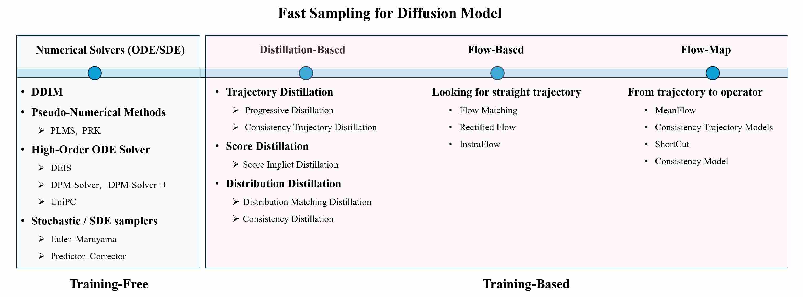
Part III — Distillation for Fast Sampling
Although higher-order ODE solvers (e.g., DPM-Solver++, UniPC) can reduce the number of denoising steps from hundreds to fewer than twenty, the computational cost remains substantial for high-resolution image synthesis and real-time applications. The ultimate goal of sampling acceleration is to achieve few-step or even single-step generation without sacrificing fidelity or diversity.
Distillation-based approaches address this challenge by compressing the multi-step diffusion process into a student model that can approximate the teacher’s distribution within only one or a few evaluations. Unlike numerical solvers, distillation learns a direct functional mapping from noise to data, thereby converting iterative denoising into an amortized process.
8. Trajectory-Based Distillation
Trajectory distillation is built on the principle distill how the teacher moves. Instead of matching only final samples, it compresses the teacher’s multi-step sampler into fewer, larger steps by teaching the student to reproduce the teacher’s transition operator \(x_{t_i}!\mapsto x_{t_{j}}\) (or an entire short segment of the trajectory).
The design philosophy is solver-centric: sampling is an algorithm, and distillation is a way to learn an approximate integrator / flow map that preserves the teacher’s path properties (stability, guidance behavior, error cancellation) under reduced NFE. Practically, this appears as step-halving curricula, multi-step-to-single-step regression targets, or direct learning of coarse-grained transitions.
8.1 Progressive Distillation
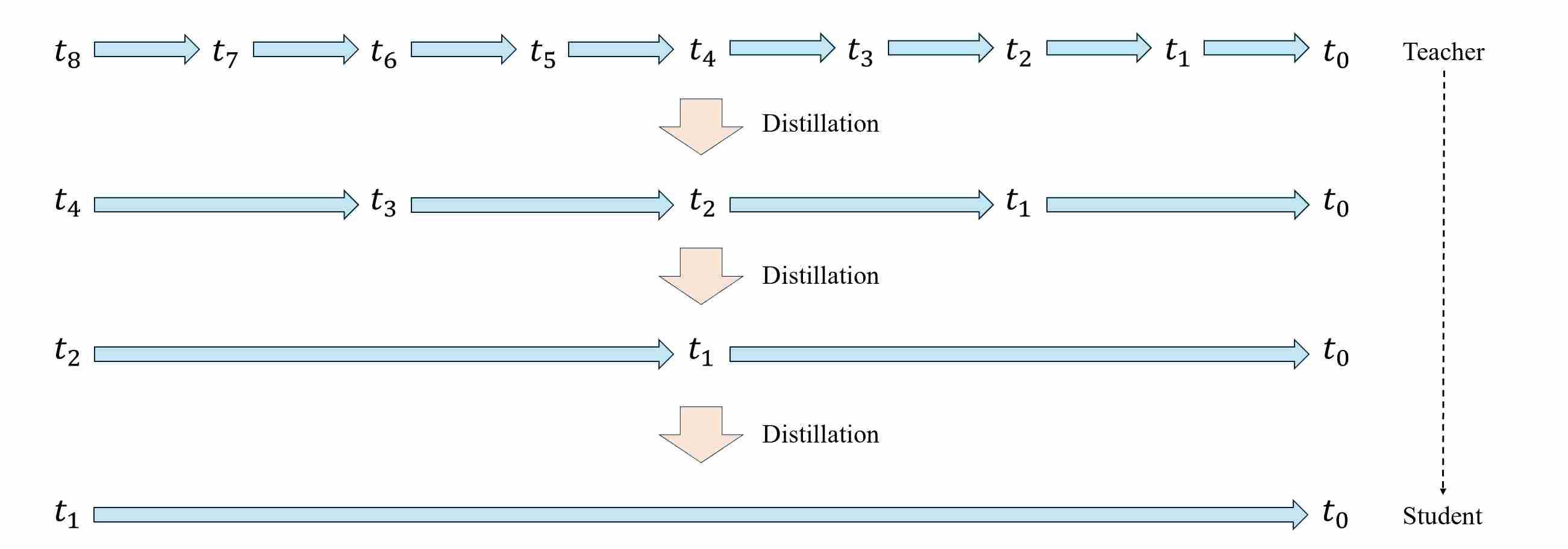
Progressive Distillation (PD) 8 compresses a pretrained “teacher” diffusion sampler that runs in $T$ steps into a “student” sampler that runs in $T/2$ steps, then recursively repeats the procedure \((T/2 \rightarrow T/4 \rightarrow \dots)\), typically reaching 4–8 steps with minimal quality loss.
Let \(\{t_n\}_{n=0}^{N}\) be a decreasing time/$\sigma$ grid with $t_0=0$ and $t_N=T$. Denote the teacher’s one-step transition (DDIM/ODE or DDPM/SDE) by
\[x_{t_{n-1}}^{\text{T}}=\Phi_\theta(x_{t_n};\,t_n \to t_{n-1}),\]where $\Phi_\theta$ is an ODE Solver. Its two-step composite
\[x_{t_{n-2}}^{\text{T}} = \Phi_\theta^{(2)}(x_{t_n};\,t_n \to t_{n-2}) = \Phi_\theta\big(\,\Phi_\theta(x_{t_n};\, t_n \to t_{n-1});\,t_{n-1}\to t_{n-2}\big).\]A student $f$ with parameters $\phi$ is trained to replace two teacher steps with one:
\[x_{t_{n-1}}^{\text{S}} = f_\phi(x_{t_n};\,t_n \to t_{n-1}) \approx \Phi_\theta^{(2)}(x_{t_n};\,t_n \to t_{n-2})\]A visualization of progressive distillation algorithm is shown as follows.
8.1.1 Target Construction and Loss Design
Training pairs are self-supervised by the teacher: Sample $x_{t_n}$ either from $\mathcal N(0,I)$ or by forward noising data \(x_0\sim p_{\text{data}}\) through \(q(x_{t_n} \mid x_0)\). Then, run two teacher steps to get the target state
\[x_{t_{n-2}}^{\text{T}}=\Phi_\theta^{(2)}(x_{t_n};\,t_n\to t_{n-2}) = x_{t_n} + \underbrace{\Delta^{(2)}_\theta(x_{t_n};\,t_n \to t_{n-2})}_{\text{Integral part from} \ t_{n} \text{ to } t_{n-2}}.\]PD can utilize different targets that we expect the student model to predict in one step from $x_t$, each corresponding to a distinct loss function. $x_{t_{n-2}}^{\text{T}$ is a simple and straightforward target that we expect the student model to predict, with this as the goal, we introduce the PD regression loss.
\[\mathcal L_{\text{state}} = \mathbb E_{x_{t_n}} \big\| f_\phi(x_{t_n};\,t_n\to t_{n-1}) - x_{t_{n-2}}^{\text{T}} \big\|_2^2\]8.1.2 Strengths and Limitations
Progressive Distillation offers an elegant and empirically robust pathway toward accelerating diffusion sampling. Its main strengths lie in its stability, modularity, and data efficiency.
- Data-free (or data-light): supervision comes from the teacher sampler itself.
- Stable and modular: each stage is a local two-step merge problem.
- Excellent trade-off at 4–8 steps: large speedups with negligible FID/IS degradation.
- Architecture-agnostic: applies to UNet/DiT backbones and both pixel/latent spaces.
However, PD also faces fundamental limitations.
Produce blurry and over-smoothed output: The MSE loss minimizes the squared difference between the prediction and the target, which mathematically drives the optimal solution toward the conditional mean of all possible teacher outputs.
- One-step limit is hard: local two-step regression accumulates errors when composed; texture/high-freq details degrade.
- Teacher-binding: student quality inherits teacher biases (guidance scale, scheduler, failure modes).
- Compute overhead: multiple PD stages plus teacher inference can approach original pretraining cost (though still typically cheaper).
8.1.3 A Canonical Training Algorithm (Template)
Below is a minimal, implementation-oriented template that captures the core algorithmic skeleton independent of specific papers.
# Progressive Distillation (PD) — 2× compression per phase
#
# teacher_step: a K-step sampler transition using teacher model θ (DDIM / PF-ODE / solver)
# student_step: a single transition using student model φ but with stride-2 (t_i -> t_{i-2})
#
# Key idea:
#   train student to match the *two-step composed teacher transition*.

def train_progressive_distillation(student, teacher, schedule, phases, optimizer):
    """
    schedule: provides alpha(t), sigma(t), and a time grid {t_0=0 < ... < t_K=T}
    phases: list of step counts, e.g., [K0, K0/2, K0/4, ..., 1]
    """
    for K in phases:
        # define teacher grid with K steps, student grid with K/2 steps (stride 2)
        t_grid = schedule.make_time_grid(K)  # descending: t_K -> ... -> t_0

        for it in range(num_train_steps_per_phase):
            # 1) sample data/noise and a random starting index n (need at least 2 teacher steps)
            x0 = sample_data()
            eps = sample_gaussian_like(x0)
            n = random_int(low=2, high=K)  # choose t_n

            # 2) form x_{t_n} by forward diffusion
            t_n = t_grid[n]
            x_tn = schedule.alpha(t_n) * x0 + schedule.sigma(t_n) * eps

            # 3) teacher: two-step composite transition t_n -> t_{n-1} -> t_{n-2}
            with no_grad():
                t_n1 = t_grid[n - 1]
                t_n2 = t_grid[n - 2]
                x_tn1_T = teacher_step(teacher, x_tn, t_n, t_n1, schedule)  # 1 step
                x_tn2_T = teacher_step(teacher, x_tn1_T, t_n1, t_n2, schedule)  # 2nd step

            # 4) student: one stride-2 transition t_n -> t_{n-2}
            x_tn2_S = student_step(student, x_tn, t_n, t_n2, schedule)

            # 5) distillation loss (L2/L1/LPIPS)
            L = distance(x_tn2_S, stopgrad(x_tn2_T))

            optimizer.zero_grad()
            L.backward()
            optimizer.step()

        # 6) after phase converges: replace teacher with student (optional)
        teacher = copy_as_teacher(student)  # or EMA(student)
Inference (Fast Generation). After progressive distillation, generation uses only the distilled student denoiser, but with a much shorter time grid. Concretely, sample an initial noise \(x_T\sim\mathcal N(0,I)\) and run the same deterministic sampler form (e.g., DDIM / PF-ODE style update) for \(K\) steps, where \(K\) is the final distilled step budget (often obtained by repeatedly halving the number of steps during training). No teacher evaluations are required at test time; the acceleration comes purely from replacing a long trajectory with a small number of coarse, student-calibrated updates.
8.2 Transitive Closure Time-Distillation
TRACT (Transitive Closure Time-Distillation) is a trajectory distillation method that generalizes binary (2-step) distillation to S-step groups, so that a teacher sampler with $T$ steps can be reduced to $T/S$ steps in one phase, and only a small number of phases (typically 2–3) are needed to reach very small step counts. 9
8.2.1 Core Idea: From Binary Merge to Transitive Closure
In a single distillation phase, the teacher schedule \(\{t_0, t_1, \dots, t_T\}\) is partitioned into contiguous groups of size $S$. Within a group, TRACT asks the student to “jump” from any time in the group directly to the group end.
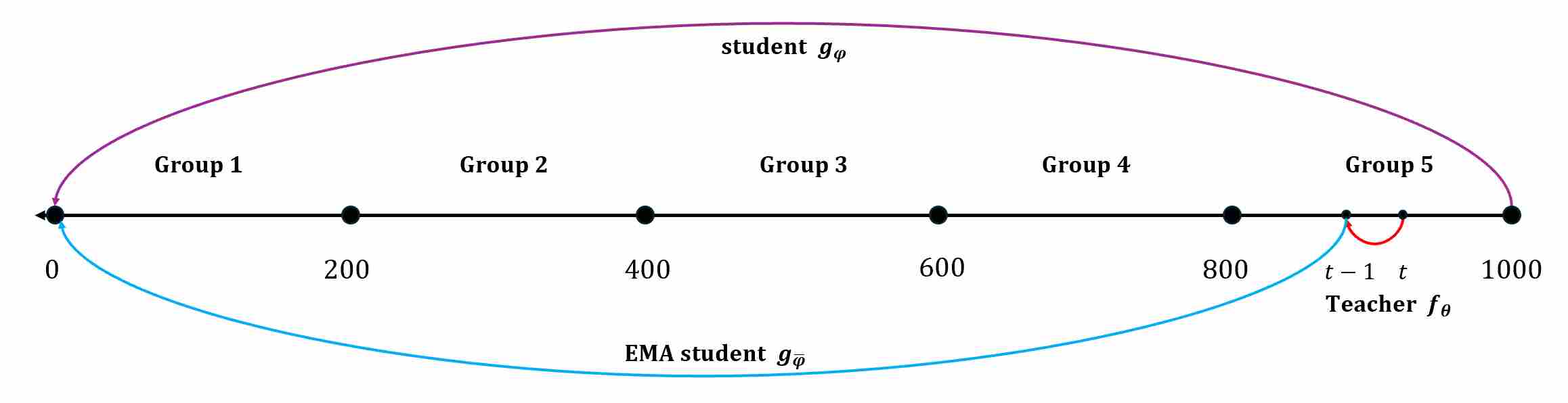
Concretely, pick a group boundary $(t_{k}, t_{k-S})$ (sampling runs backward), and consider any intermediate $t_{k-i}$ with $i \in {0,\dots,S-1}$. We define:
Teacher one-step transition (e.g., DDIM / ODE step):
\[x_{t_{k-i-1}}^{\mathrm T} = f_{\theta}(x_{t_{k-i}};\,t_{k-i}\to t_{k-i-1}).\]Student long jump transition (same network, but larger time stride):
\[x_{t_{k-S}}^{\mathrm S} = g_{\varphi}(x_{t_{k-i}};\,t_{k-i}\to t_{k-S}).\]
If we naively enforced the “jump-from-anywhere” constraint, training would require multiple student calls per example (one for each possible $t_{k-i}$), which is expensive.
\[g_\varphi(x_{t_{k-i}};\,t_{k-i}\to t_{k-S})\;=\;f_{\theta}(\ldots f_{\theta}(x_{t_{k-i}};\,t_{k-i}\to t_{k-i-1})).\]TRACT resolves this by introducing a self-teacher $g_{\bar\varphi}$, an EMA of the student, and enforces transitive closure via a recurrence: the “long jump” from $t_{k-i}$ to $t_{k-S}$ is defined by composing
- One teacher step: one teacher step from $t_{k-i}$ to $t_{k-i-1}$ and
- Bootstrapping with EMA-student: one EMA-student jump from $t_{k-i-1}$ to $t_{k-S}$.
A simple way to write the training target state is:
If $i=S-1$ (already adjacent to the group end), the teacher can provide the endpoint directly:
\[x_{t_{k-S}}^{\mathrm T}=f_{\theta}(x_{t_{k-S+1}};\,t_{k-S+1}\to t_{k-S}).\]Otherwise (general case), use the self-teacher recurrence:
\[x_{t_{k-S}}^{\mathrm T} = g_{\bar\varphi}\Big( f_{\theta}(x_{t_{k-i}};\,t_{k-i}\to t_{k-i-1}); \,t_{k-i-1}\to t_{k-S}\Big).\]
8.2.2 Target Construction and Objective
Like PD/BTD, TRACT can be implemented with a signal-prediction (i.e., $\hat x_0$) network. The student network itself still takes the standard diffusion inputs $(x_t, t, c)$ and predicts $\hat x_0$; the “destination” $t_{k-S}$ is used only in the deterministic update (it selects the coefficients). 9
Let $x_t=\sqrt{\alpha_t}x_0+\sqrt{1-\alpha_t}\,\epsilon$ (VP parameterization), so during training we can compute the exact noise:
\[\epsilon = \frac{x_t-\sqrt{\alpha_t}\,x_0}{\sqrt{1-\alpha_t}}.\]Given the target endpoint state $x_{t_{k-S}}^{\mathrm T}$ (constructed above), we choose the target clean signal $x_0^{\star}$ so that a DDIM-style deterministic jump from $t$ to $t_{k-S}$ using the same $\epsilon$ reproduces $x_{t_{k-S}}^{\mathrm T}$:
\[x_0^{\star} = \frac{x_{t_{k-S}}^{\mathrm T} - \sqrt{1-\alpha_{t_{k-S}}}\,\epsilon}{\sqrt{\alpha_{t_{k-S}}}}.\]Then the student is trained by a standard regression (optionally with the usual DDIM/VP weighting):
\[\mathcal L_{\text{TRACT}} = \mathbb E\Big[ \lambda(t)\,\big\| \hat x_{0,\phi}(x_t,t,c) - x_0^{\star}\big\|_2^2 \Big].\]This view also clarifies a common confusion: TRACT does not require the model to explicitly take an endpoint $s$ as input. The network remains a standard $\hat x_0(x_t,t,c)$ predictor; the chosen stride (e.g., “jump to group end”) is realized by plugging $\hat x_0$ into a deterministic solver update with the corresponding $(\alpha_t,\alpha_s)$. 9
Important: why the target construction enforces $x_t$ and $x_s$ lie on the same DDIM trajectory
In TRACT, the supervision target is constructed under the DDIM (η = 0) trajectory model, where a trajectory is characterized by a shared latent noise ε (and a shared clean signal x₀) across time. Concretely, DDIM assumes that along a deterministic path we can write, for any two times t > s, $$ x_t = \sqrt{\gamma_t}\,x_0 + \sqrt{1-\gamma_t}\,\epsilon,\qquad x_s = \sqrt{\gamma_s}\,x_0 + \sqrt{1-\gamma_s}\,\epsilon, $$ with the same ε. TRACT then chooses the target x̂ (an x₀-prediction target) by eliminating ε and solving for x₀, yielding a closed-form x̂ that makes $(x_t, x_s)$ consistent with one DDIM trajectory. $$ \hat x = \frac{ x_s\sqrt{1-\gamma_t}-x_t\sqrt{1-\gamma_s} }{ \sqrt{\gamma_s}\sqrt{1-\gamma_t}-\sqrt{\gamma_t}\sqrt{1-\gamma_s} }, $$ The regression loss pushes the student $g_φ(x_t,t)$ toward this x̂; equivalently, it enforces that the inferred noise $$ \hat\epsilon=\frac{x_t-\sqrt{\gamma_t}\,g_\phi(x_t,t)}{\sqrt{1-\gamma_t}}, $$ is the same noise that reproduces x_s under DDIM reconstruction. Therefore, the target construction does not merely fit x₀ in isolation—it explicitly enforces that x_t and x_s share the same latent noise and hence lie on the same deterministic DDIM path.
8.2.3 TRACT vs. Progressive Distillation (Key Differences)
- Stride: PD enforces a fixed compression ratio of 2 per phase; TRACT uses an arbitrary group size $S$, enabling much larger stride per phase. 9
- Constraint form: PD matches a two-step teacher composition with a one-step student; TRACT enforces a transitive-closure recurrence over a group, so that jumps from interior points are consistent with jumps from later points. 9
- Teacher quality: PD’s “teacher of the next phase” is the previous student; TRACT’s recurrence uses an EMA self-teacher inside a phase to stabilize targets while avoiding many generations. 9
- Compute: With the recurrence, each training sample needs only one teacher step + one self-teacher jump, rather than multiple student evaluations across group positions. 9
8.2.4 A Canonical Training Algorithm (Template)
Below is a minimal, implementation-oriented template that captures the core algorithmic skeleton independent of specific papers.
# TRACT (Transitive Closure Time-Distillation)

# Inputs:
#   teacher: The original pretrained model (frozen)
#   student: The model being trained
#   student_ema: EMA copy of the student (provides stable targets)
#   S: Group size (striding factor)

for each training step:
    # 1. Sample trajectory parameters
    x0 ~ p_data(x)
    # Sample a group boundary index k (e.g., t_k is the destination)
    # Sample an intermediate point i within the group [k, k+S]
    k ~ ...
    i ~ Uniform({0, ..., S-1})
    t_start = t_{k+i}
    t_end   = t_k

    # 2. Forward diffusion to t_start
    epsilon ~ N(0, I)
    x_start = sqrt(alpha[t_start]) * x0 + sqrt(1 - alpha[t_start]) * epsilon

    # 3. Construct Target (Transitive Closure)
    with no_grad:
        # a) Take ONE step with the frozen Teacher
        #    t_{k+i} -> t_{k+i-1}
        x0_teach = teacher(x_start, t_start)
        x_prev = DDIM_Step(x_start, x0_teach, t_start, t_{k+i-1})

        # b) Bridge the rest with EMA Student
        #    t_{k+i-1} -> t_k
        if i == 0:
            # If we are already adjacent to target, teacher step is enough
            x_target_state = x_prev
        else:
            # Otherwise, use EMA student to jump the gap
            x0_ema = student_ema(x_prev, t_{k+i-1})
            x_target_state = DDIM_Step(x_prev, x0_ema, t_{k+i-1}, t_end)

        # c) Convert state target back to implied x0 target (using t_start noise definition)
        #    This ensures x_start and x_target_state lie on same DDIM trajectory
        x0_target = Solve_x0_from_DDIM(x_start, x_target_state, t_start, t_end)

    # 4. Student Prediction
    pred_x0 = student(x_start, t_start)

    # 5. Regression Loss
    L = MSE(pred_x0, x0_target)

    update(student, L)
    update_ema(student_ema, student)
Inference (Fast Generation). Inference with TRACT is extremely efficient because the student has learned the “transitive closure” of the trajectory, enabling it to perform “long jumps” directly. For a 1-step distillation, you simply input Gaussian noise $x_T$ and the student outputs the clean sample $x_0$ immediately.
For multi-step variants (e.g., 2 steps), you follow the specific strided schedule determined by the group size $S$ during training (e.g., jumping from $T \to T-S, \dots, \to , \dots$ and then final $0$). This bypasses the need for the EMA self-teacher or the original teacher during inference.
8.3 Guided Distillation
So far, our discussion implicitly assumes an unguided diffusion model, where each sampling step requires one network evaluation. However, modern high-quality text-to-image systems heavily rely on classifier-free guidance (CFG), which doubles per-step cost by evaluating: one for a conditional model (\(\epsilon_{c}\), with prompt / class), and another for an unconditional model (\(\epsilon_{\phi}\), null prompt), then mixing them with a guidance scale.
\[\epsilon_{total} = \epsilon_{\phi} + g\cdot(\epsilon_{c} - \epsilon_{\phi} )\]This creates a second bottleneck orthogonal to “number of steps”: even if you distill \(N\!\to\!4\) steps, CFG still costs roughly $2\times 4$ forward passes. Guided distillation 10 tackles both axes:
distill “two-model guidance” into one student (remove the 2× factor),
then apply progressive / trajectory distillation to reduce steps further.
8.3.1 Stage-One: Distill the Guidance Operator
Let the teacher provide two predictions at time $t$: a conditional one \(\hat x^{c}_{\theta}(z_t)\) and an unconditional one \(\hat x_{\theta}(z_t)\). CFG combines them into a guided prediction at guidance strength $w$:
\[\hat x^{w}_{\theta}(z_t) = (1+w)\,\hat x^{c}_{\theta}(z_t) - w\,\hat x_{\theta}(z_t).\]The key idea is to train a single student \(\hat x_{\eta_1}(z_t, w)\) (also conditioned on context $c$) to directly regress this combined target for a range of $w$ values:
\[\min_{\eta_1}\ \mathbb E_{w\sim\mathcal U[w_{\min},w_{\max}],\ t\sim\mathcal U[0,1],\ x\sim p_{\text{data}}} \Big[ \omega(t)\ \big\|\hat x_{\eta_1}(z_t,w) - \hat x^{w}_{\theta}(z_t)\big\|_2^2 \Big].\]This removes the “two-network per step” overhead while retaining the quality–diversity knob via $w$-conditioning. 10
8.3.2 Stage-Two: Distill Sampling Steps (Progressive / Binary)
After stage-one, the student already matches the guided teacher prediction at each time, but still requires many steps if we sample with the original schedule. Stage-two applies standard step distillation: train a student to match a two-step DDIM trajectory segment of the (guided) teacher in one step, then repeat to halve the number of steps again (initializing each new student from its teacher). 10
Conceptually, guided distillation is therefore “trajectory distillation” in two layers:
Operator distillation (guidance): distill the combination rule \((\hat x^c,\hat x)\mapsto \hat x^w\) into a single network.
Time distillation (steps): distill multi-step solver trajectories into fewer steps.
In practice, the biggest win often comes from stage-one (saving ~2× compute per step), while stage-two provides the additional “few-step” acceleration. 10
8.3.3 A Canonical Training Algorithm (Template)
Below is a minimal, implementation-oriented template that captures the core algorithmic skeleton independent of specific papers.
Guided Distillation (Stage 1):
# Guided Distillation (Stage 1: Distilling CFG)

# Inputs:
#   teacher: Pretrained model (capable of conditional & unconditional)
#   student: Model taking w (guidance scale) as extra input
#   w_min, w_max: Range of guidance scales to distill

for each training step:
    # 1. Prepare data
    x0, c ~ p_data(x, c) # Image and Text Condition
    t ~ Uniform(0, T)
    epsilon ~ N(0, I)
    x_t = diffuse(x0, t, epsilon)

    # 2. Sample a random guidance scale w
    w ~ Uniform(w_min, w_max)

    # 3. Compute Teacher's Guided Output
    with no_grad:
        # Get conditional and unconditional noise predictions
        eps_cond = teacher(x_t, t, c)
        eps_uncond = teacher(x_t, t, null_c)

        # Apply Classifier-Free Guidance formula
        eps_target = eps_uncond + w * (eps_cond - eps_uncond)

        # (Optional) Convert to x0 space if distilling x0
        x0_target = predict_x0_from_eps(x_t, t, eps_target)

    # 4. Student Prediction
    # Student explicitly takes 'w' as conditioning input
    x0_student = student(x_t, t, c, w)

    # 5. Loss
    L = MSE(x0_student, x0_target)

    update(student, L)
Guided Distillation (Stage 2):
# Guided Distillation — Stage Two: distill sampling steps (PD/TRACT/etc.)
#
# Treat the stage-one guided student as "teacher sampler" (with guidance baked in),
# then perform standard step-distillation to reduce step count.

def train_guided_step_distill(student_fewstep, teacher_guided_student, schedule, phases, optimizer):
    # identical skeleton to PD, except teacher_step uses teacher_guided_student
    # and student_step uses student_fewstep (both already include guidance behavior).
    train_progressive_distillation(
        student=student_fewstep,
        teacher=teacher_guided_student,
        schedule=schedule,
        phases=phases,
        optimizer=optimizer
    )
Inference (Fast Generation). The primary advantage during inference is the elimination of the double-batching requirement inherent in Classifier-Free Guidance. Instead of evaluating the model twice (once for $\epsilon_{\text{cond}}$ and once for $\epsilon_{\text{uncond}}$) and manually combining them, you feed the noise $x_t$, the text condition $c$, and your desired guidance scale $w$ (e.g., $w=7.5$) directly into the student model. The student outputs the pre-combined, guided result in a single forward pass per timestep, effectively doubling the inference speed for any given sampler (e.g., DDIM or Euler).
9. Adversarial-Based Distillation
Adversarial distillation follows the principle “distill fast realism by adding a critic.” The central belief is that ultra-few-step (especially one-step) generators suffer from perceptual artifacts that are not fully penalized by teacher-matching losses alone, so a discriminator provides a complementary signal that sharply enforces high-frequency realism and data-manifold alignment.
The philosophy is hybrid: keep the teacher as a semantic / distributional supervisor while using adversarial training as a perceptual regularizer that compensates for the limited iterative correction budget. In practice, adversarial objectives are rarely used alone—they are layered on top of score/disttribution/trajectory losses to stabilize training and improve texture fidelity.
9.1 Adversarial Diffusion Distillation
While Progressive Distillation (Sec. 8) compresses multi-step sampling through supervised teacher-student regression, it still depends on explicit trajectory matching: the student must imitate the teacher’s denoising transitions.
Adversarial Diffusion Distillation (ADD) 11 proposes a fundamentally different perspective: rather than minimizing a reconstruction distance between teacher and student trajectories, the student is trained adversarially to generate outputs that are indistinguishable from real data, while remaining consistent with the diffusion process implied by the teacher.
9.1.1 Motivation: From Trajectory Matching to Perceptual Realism
Trajectory-based distillation implicitly assumes the teacher path is a good proxy for perceptual quality. But under aggressive compression (e.g., 1–4 steps), supervised matching tends to reproduce the teacher’s mean-like behavior, leading to blurred edges and weak high-frequency details. ADD injects a critic that explicitly penalizes “off-manifold” artifacts, while the teacher still anchors the student to the diffusion prior and the condition (text/image guidance).
9.1.2 Principle and Formulation
Let $x_T\sim\mathcal N(0,I)$ denote the initial noise and $\Phi_\text{teacher}$ the full diffusion sampler of teacher model (DDIM, ODE, or PF-ODE). ADD seeks to train a student generator $G_\phi(x_K;\,K\to 0)$ that approximates the teacher’s final output $\Phi_\text{teacher}(x_T;\,T\to0)$ in $K$ step ($K$ is small, \(K \ll T\)), while simultaneously fooling an adversarial discriminator $D_\psi(x)$. Its loss function consists of two parts.
1. Teacher Consistency Loss. To maintain semantic alignment with the diffusion manifold, ADD retains a lightweight teacher consistency term:
\[\mathcal L_{\text{distill}} = \mathbb E_{x_T} \left[\|G_\phi(x_K;\,K\to 0) - \Phi_\text{teacher}(x_T;\,T\to 0)\|_2^2 \right].\]This term ensures that the student’s outputs lie near the teacher’s sample space, preserving the diffusion prior.
2. Adversarial Loss. A discriminator $D_\psi$ is trained to differentiate real data $x_0 \sim p_\text{data}$ from generated samples $G_\phi(x_K;\,K\to 0)$. The standard non-saturating (or hinge) GAN loss is adopted:
\[\mathcal L_{\text{adv}}^G = -\mathbb E_{x_T\sim \mathcal N(0,I)} [\log D_\psi(G_\phi(x_K;\,K\to 0))].\]By optimizing $\mathcal L_{\text{adv}}^G$ jointly with $\mathcal L_{\text{distill}}$, the student learns to generate visually realistic samples that also align with the teacher’s denoising manifold.
The overall training objective combines both components with a weighting $\lambda_{\text{adv}}$:
\[\mathcal L_{\text{ADD}} = \mathcal L_{\text{distill}} +\lambda_{\text{adv}}\, \mathcal L_{\text{adv}}^G.\]During training, the discriminator $D_\psi$ is updated alternately to maximize $\mathcal L_D$.
\[\mathcal L_D = -\,\mathbb E_{x_0\sim p_\text{data}} [\log D_\psi(x_0)] -\,\mathbb E_{x_T\sim \mathcal N(0,I)} [\log(1 - D_\psi(G_\phi(x_K;\,K\to 0)))]\]9.1.3 Implementation Mechanism
The training procedure can be express in the following figure.
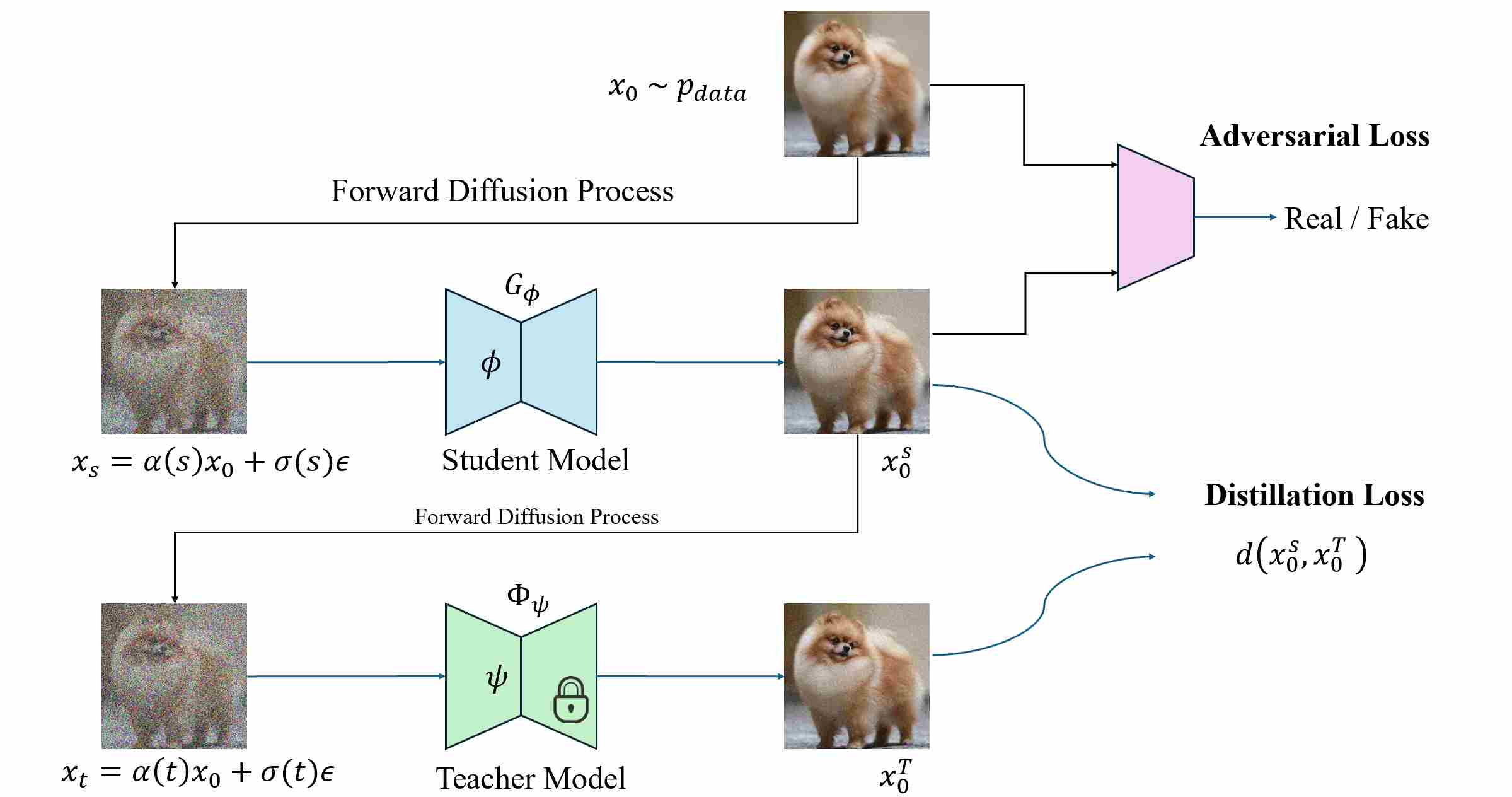
During training, let $x_0 \sim p_{\text{data}}$.
Step 1: utilize forward diffusion process to add noise to clean image $x_0$.
\[x_s = \alpha(s)x_0 + \sigma(s)\epsilon ,\qquad \epsilon \sim \mathcal N(0,I).\]where $0 < s \leq K $.
step 2: The student first performs a s-step denoising:
\[x_0^{S}=G_\phi(x_s; s\to 0)\]This represents the image the student would produce during inference.
step 3: Instead of drawing real data $x_0$ again from the dataset, ADD reuses the student’s own output $x_0^{S}$ and applies forward diffusion:
\[x_t = \alpha(t) x_0^{S} + \sigma(t)\epsilon^{'} , \qquad \epsilon^{'} \sim \mathcal N(0,I).\]where $0 < t \leq T $. This design is crucial—the teacher is conditioned on the student’s current distribution rather than on real data. By doing so, the teacher supervises exactly the domain that the student will visit at inference time, forming a closed-loop, on-policy distillation process.
step 4: The teacher diffusion model, typically a pretrained DDIM or PF-ODE sampler, now starts from $x_t$ and performs full multi-step denoising:
\[x_0^{T}=\Phi_{\text{teacher}}(x_t;\,t\to 0),\]yielding a high-quality reconstruction of what that noisy sample should look like under the teacher’s diffusion dynamics.
step 5: The pair $(x_0^{S},,x_0^{T})$ defines the distillation target, while an adversarial discriminator evaluates realism relative to real data $x_0 \sim p_{\text{data}}$.
At inference, only the student is used: one forward pass from Gaussian noise $x_T$ directly yields $x_0^S$. The teacher is entirely discarded.
9.1.4 A Canonical Training Algorithm (Template)
Below is a minimal, implementation-oriented template that captures the core algorithmic skeleton independent of specific papers.
# ADD — Adversarial Diffusion Distillation (on-policy)
#
# student: G_φ(x_s; s->0)  (few-step sampler or 1-step)
# teacher: Φ_teacher(x_t; t->0) (full sampler)
# discriminator: D_ψ(·)

def train_add(student_G, teacher_sampler, discriminator_D, schedule, optimizer_G, optimizer_D,
              lambda_adv=1.0, s_max_steps=K_student):

    for it in range(num_train_steps):
        # --------- sample real data ----------
        x0_real = sample_data()

        # --------- Step 1: forward diffuse to x_s ----------
        s = sample_time_in_range(0, s_max_steps)  # your "0 < s <= K"
        eps = sample_gaussian_like(x0_real)
        x_s = schedule.alpha(s) * x0_real + schedule.sigma(s) * eps

        # --------- Step 2: student denoise (inference-like) ----------
        x0_S = student_G(x_s, s, 0, schedule)  # denotes G_φ(x_s; s->0)

        # --------- Step 3: re-noise student output (on-policy) ----------
        t = sample_time_in_range(0, T)
        eps2 = sample_gaussian_like(x0_S)
        x_t = schedule.alpha(t) * x0_S + schedule.sigma(t) * eps2

        # --------- Step 4: teacher denoise from x_t ----------
        with no_grad():
            x0_T = teacher_sampler(x_t, t, 0, schedule)  # Φ_teacher(x_t; t->0)

        # --------- Step 5: distillation + adversarial ----------
        # distillation/regression term (L2/L1/LPIPS etc.)
        L_distill = distance(x0_S, stopgrad(x0_T))

        # GAN losses (non-saturating)
        #   L_adv^G = -E log D(x0_S)
        #   L_D     = -E log D(x0_real) - E log(1 - D(x0_S))
        D_real = discriminator_D(x0_real)
        D_fake = discriminator_D(x0_S.detach())

        L_D = -(log(D_real) + log(1.0 - D_fake)).mean()

        optimizer_D.zero_grad()
        L_D.backward()
        optimizer_D.step()

        # generator adversarial
        D_fake_for_G = discriminator_D(x0_S)
        L_adv_G = -log(D_fake_for_G).mean()

        L_G = L_distill + lambda_adv * L_adv_G

        optimizer_G.zero_grad()
        L_G.backward()
        optimizer_G.step()
Inference (Fast Generation). ADD is specifically designed for single-step or ultra-low-step generation. At inference, the discriminator and the teacher model are completely discarded. You simply draw random Gaussian noise $x_T$ and pass it through the student model once. Thanks to the adversarial training, the student directly outputs a high-fidelity, perceptually sharp image $x_0$ without needing an iterative denoising loop or a complex scheduler. If trained for multi-step (e.g., 4 steps), you would run the student 4 times, but for the standard 1-step ADD, it is a direct mapping from noise to image.
9.2 Progressive Adversarial Diffusion Distillation (PADD)
Progressive Adversarial Diffusion Distillation (PADD) 12 can be read as a targeted “fix” of ADD/SDXL-Turbo-style adversarial distillation: rather than training the student to jump to the ODE endpoint at every step (and then re-noising again for multi-step sampling), PADD trains a student that directly approximates the teacher’s probability flow transition between two timesteps, and uses an adversarial signal to recover sharpness.
Conceptually, PADD = (i) progressive solver distillation (stability) + (ii) flow-preserving adversarial constraint (compatibility) + (iii) mode-coverage relaxation (artifact mitigation).
9.2.1 Principle: distill a flow-preserving jump operator
Let a teacher diffusion sampler define a deterministic probability-flow (e.g., DDIM / PF-ODE) update operator. For training, we sample a clean latent/image pair \((x_0, c)\) and noise \(\epsilon\sim\mathcal N(0,I)\), then jump to an arbitrary timestep \(t\) to re-noise:
\[x_t = \mathrm{forward}(x_0,\epsilon,t).\]To distill a large step of size \(n_s\), the teacher rolls out \(n\) small solver steps (step size \(s\), so that \(n_s=n\cdot s\)) to obtain the target \(x_{t-n_s}\). In “direction-field” form (as in PF-ODE / DDIM-style updates), denote the teacher field by \(u_t = f_{\text{teacher}}(x_t,t,c)\), and a deterministic move operator \(\mathrm{move}(\cdot)\) that maps \((x_t,u_t)\) to a new time \(t'\):
\[\begin{aligned} u_t & = f_{\text{teacher}}(x_t,t,c),\\[10pt] \Longrightarrow\quad x_{t-s} & = \mathrm{move}(x_t,u_t,t,t-s), \\[10pt] \Longrightarrow\quad \quad \quad \ldots \\[10pt] \Longrightarrow\quad x_{t-n_s} & = \mathrm{move}(x_{t-(n-1)s},u_{t-(n-1)s},t-(n-1)s,t-n_s). \end{aligned}\]The student is trained to predict a single field \(\hat u_t=f_{\text{student}}(x_t,t,c)\) that directly “jumps” to \(t-n_s\):
\[\hat u_t = f_{\text{student}}(x_t,t,c),\qquad \hat x_{t-n_s}=\mathrm{move}(x_t,\hat u_t,t,t-n_s).\]A baseline progressive distillation would minimize the regression objective
\[\mathcal L_{\text{mse}} = \left\|\hat x_{t-n_s}-x_{t-n_s}\right\|_2^2.\]However, in the few-step regime, pure MSE tends to yield overly smoothed / blurry results. PADD replaces the regression supervision with an adversarial objective while keeping the distillation target tied to the teacher’s flow.
9.2.2 Flow-preserving conditional adversarial objective
PADD defines a discriminator that classifies whether \(x_{t-n_s}\) comes from the teacher transition or from the student transition, conditioned on the same starting state \(x_t\) (and prompt \(c\)):
\[D(x_t,x_{t-n_s},t,t-n_s,c)\in[0,1].\]With non-saturating GAN losses, the teacher sample is labeled “real” and the student sample is labeled “fake”. Define
\[p = D(x_t,x_{t-n_s},t,t-n_s,c),\qquad \hat p = D(x_t,\hat x_{t-n_s},t,t-n_s,c).\]Then the discriminator loss and generator (student) loss are:
\[\mathcal L_D = -\log(p) - \log(1-\hat p),\] \[\mathcal L_G = -\log(\hat p).\]Why conditioning on (x_t) matters. Under probability-flow sampling, the teacher’s mapping from \(x_t\) to \(x_{t-n_s}\) is (approximately) deterministic. If the discriminator sees both \(x_t\) and the candidate next state, it is forced to judge whether the pair \((x_t\!\to\!x_{t-n_s})\) follows the teacher’s same flow; consequently, the student must imitate the same flow to fool \(D\). This is the key ingredient for (a) multi-step sampling without re-noising hacks and (b) better compatibility with LoRA / ControlNet-like modules that were trained under the teacher’s dynamics.
9.2.3 Discriminator design in latent space
Instead of using an external image encoder (e.g., DINO) and discriminating only at \(t=0\), PADD reuses the teacher diffusion U-Net encoder as a discriminator backbone (latent-native, timestep-aware, prompt-aware). Concretely, let \(d(\cdot)\) be the copied encoder+midblock. PADD passes \(x_{t-n_s}\) and \(x_t\) through the shared backbone, concatenates their midblock features, and applies a small head:
\[D(x_t,x_{t-n_s},t,t-n_s,c) \equiv \sigma\Big(\mathrm{head}\big(d(x_{t-n_s},t-n_s,c),\; d(x_t,t,c)\big)\Big).\]This makes the discriminator scalable to high resolutions and valid across noise levels.
9.2.4 Relax mode coverage to remove “Janus” artifacts
A subtle but important phenomenon in adversarial distillation is the Janus artifact: the teacher can make sharp layout changes between nearby noise inputs, but a small-step student lacks the capacity to reproduce such “sudden turns”. Under a strictly flow-preserving adversarial objective, the student may sacrifice semantic correctness to preserve sharpness, producing conjoined / duplicated body parts.
PADD mitigates this by relaxing the flow-preservation constraint after the main adversarial training: it finetunes with a discriminator that no longer conditions on \(x_t\),
\[D'(x_{t-n_s},t-n_s,c)\equiv \sigma\Big(\mathrm{head}(d(x_{t-n_s},t-n_s,c))\Big),\]so the objective emphasizes per-sample realism more than strict transition consistency. In practice, at every progressive stage, PADD trains first with \(D\) (conditional, flow-preserving) and then finetunes with \(D'\) (unconditional, artifact removal).
9.2.5 A Canonical Training Algorithm (Template)
Below is a minimal, implementation-oriented template that captures the core algorithmic skeleton independent of specific papers.
Stage A: Warm-up (MSE distillation)
# PADD — Progressive Adversarial Diffusion Distillation
#
# Key objects:
#   teacher f_T (frozen), student f_S (trainable)
#   forward(x0, ε, t) -> x_t
#   δ_T: teacher transition (rollout)     x_t -> x_{t'}^T
#   δ_S: student transition (one-jump)    x_t -> x̂_{t'}
#   D:  conditional discriminator  D(x_t, x_{t'}, t, t', c)
#   D': unconditional discriminator D'(x_{t'}, t', c)
#
# Non-saturating GAN:
#   L_D  = -log D(real) - log(1 - D(fake))
#   L_G  = -log D(fake)
#
# Stage plan (paper recipe): 128→32 (MSE), then 32→8→4→2→1 (GAN), each stage: D then D'

def PADD_train_template():
    # ------------------------------------------------------------
    # Stage A: Warm-up (MSE distillation), e.g., 128 -> 32
    # ------------------------------------------------------------
    init student f_S ← teacher f_T
    for it in range(N_mse):
        sample (x0, c), sample ε, sample adjacent (t > t') from grid(32)
        x_t = forward(x0, ε, t)                  # optional: if t==T use pure noise (schedule fix)
        x_{t'}^T = δ_T(x_t, t→t', c)             # teacher rollout target
        x̂_{t'}   = δ_S(x_t, t→t', c)             # student one-jump
        update f_S by minimizing ||x̂_{t'} - stopgrad(x_{t'}^T)||^2
Stage B: Conditional Progressive Adversarial Distillation
# Given: teacher (frozen), student (trainable), discriminator D (trainable)
# Hyper: n, s  (so jump = n*s), timestep sampler, noise sampler

for each iteration:
    x0, c = sample_data()              # latent of image + text condition
    t = sample_timestep_for_this_stage()
    eps = torch.randn_like(x0)

    # (optional) schedule fix: if t == T, use pure noise as input
    xt = Forward(x0, eps, t)           # Eq(24) hack for t=T
    # teacher target: run n small steps (size s) to reach t-ns
    x_teacher = teacher_multistep(teacher, xt, t, n, s, c)   # gives x_{t-ns}
    # student one jump
    x_fake = student_jump(student, xt, t, n, s, c)           # gives x̂_{t-ns}

    # --- update discriminator (non-saturated GAN) ---
    p_real = D(xt, x_teacher, t, t-n*s, c)
    p_fake = D(xt, x_fake.detach(), t, t-n*s, c)
    L_D = -log(p_real) - log(1 - p_fake)
    step(D, L_D)

    # --- update student (generator) ---
    p_fake_for_G = D(xt, x_fake, t, t-n*s, c)
    L_G = -log(p_fake_for_G)
    step(student, L_G)
Stage B: UnConditional Progressive Adversarial Distillation
# After conditional stage converges
for each iteration:
    x0, c = sample_data()
    t = sample_timestep_for_this_stage()
    eps = randn()

    xt = Forward(x0, eps, t)
    x_teacher = teacher_multistep(...)
    x_fake = student_jump(...)

    # discriminator without conditioning on xt
    p_real = D_prime(x_teacher, t-n*s, c)
    p_fake = D_prime(x_fake.detach(), t-n*s, c)
    L_Dp = -log(p_real) - log(1 - p_fake)
    step(D_prime, L_Dp)

    p_fake_for_G = D_prime(x_fake, t-n*s, c)
    L_G = -log(p_fake_for_G)
    step(student, L_G)
Inference (few-step sampling).
Given a step schedule \(T=t_S > t_{S-1}>\cdots>t_0=0\) and initial noise \(x_T\sim\mathcal N(0,I)\), apply the student as a solver:
No “add-noise-again” is needed: multi-step inference follows the same learned probability flow transitions by construction.
Overall, PADD can be summarized as: progressively distill the solver (stability) + constrain the learned dynamics (compatibility) + use adversarial feedback (sharpness).
9.3 Latent Adversarial Diffusion Distillation (LADD)
ADD’s projected discriminator is effective, but for latent diffusion models it introduces a major inefficiency: to compute an image-space adversarial loss (e.g., on DINO features), one must repeatedly decode latents into pixels, which is expensive and memory-heavy. Latent Adversarial Diffusion Distillation (LADD) 13 addresses this by redesigning the discriminator pipeline to be latent-native and teacher-feature-based, enabling high-resolution training for modern large latent diffusion transformers (e.g., SD3 / MMDiT). At a high level, LADD introduces two key modifications:
- Unify discriminator and teacher: use the teacher diffusion model itself as the feature extractor for adversarial training.
- Leverage synthetic data: teacher-generated (prompt, latent) pairs can improve text alignment so much that an explicit distillation term becomes less important.
9.3.1 Unifying teacher and discriminator via multi-layer token features
Work purely in latent space. Let \(z_0\) be a clean latent, and define forward noising in latent space:
\[z_{\hat t} = \alpha(\hat t)z_0 + \sigma(\hat t)\epsilon,\qquad \epsilon\sim\mathcal N(0,I).\]A core LADD design is: sample a teacher evaluation noise level \(\hat t\) from a logit-normal distribution \(\pi(\hat t)\). Then apply the teacher to \(z_{\hat t}\) and extract the full token sequence after each attention block. Denote teacher features (token sequences / hidden states) at depth \(k\) by
\[F_k(z_{\hat t},\hat t,c)\in\mathbb R^{N\times d}.\]On each \(F_k\), attach an independent discriminator head \(h_k\) to output a binary real/fake probability:
\[D_k(z_{\hat t},\hat t,c)=\sigma\Big(h_k(F_k(z_{\hat t},\hat t,c),\; \hat t,\; \mathrm{pool}(c))\Big).\]Important: “multi-head discriminator” here does not mean multi-class classification. Each head is still a binary classifier; “multi-head” means many binary heads at multiple depths, providing multi-scale, noise-aware adversarial gradients (Projected-GAN style, but using generative teacher features instead of a discriminative encoder).
9.3.2 Noise-aware conditioning as a knob
Because features come from a diffusion teacher, they vary systematically with \(\hat t\): high-noise features emphasize global structure; low-noise features emphasize texture. Therefore, changing \(\pi(\hat t)\) directly changes what the discriminator focuses on—acting as a knob to trade off global coherence vs fine details. This is conceptually similar to loss reweighting across timesteps in diffusion training, but now implemented through adversarial feedback.
9.3.3 Objective: multi-head adversarial loss (and optional distillation)
Let “real” latents come from data (VAE-encoded) or teacher-generated latents, and “fake” latents come from the student. After noising both to \(\hat t\), compute per-head real/fake probabilities \(D_k^{\text{real}}, D_k^{\text{fake}}\). A convenient implementation uses the non-saturating GAN loss per head:
\[\mathcal L_D = \sum_k\Big(-\log D_k^{\text{real}} - \log(1-D_k^{\text{fake}})\Big),\] \[\mathcal L_G^{\text{adv}} = \sum_k\Big(-\log D_k^{\text{fake}}\Big).\]Optionally, include a lightweight distillation constraint (e.g., MSE between student and teacher denoised predictions) to stabilize training on real data:
\[\mathcal L_{\text{distill}} = \mathbb E\left[\|\,\mathrm{Student}(z_{\hat t},\hat t,c) - \mathrm{Teacher}(z_{\hat t},\hat t,c)\,\|_2^2\right].\]In practice, LADD observes that with teacher-synthesized data, adversarial training alone can be sufficient and the auxiliary \(\mathcal L_{\text{distill}}\) becomes less critical.
9.3.4 A Canonical Training Algorithm (Template)
Below is a minimal, implementation-oriented template that captures the core algorithmic skeleton independent of specific papers.
# Latent Adversarial Diffusion Distillation (LADD)

# Inputs:
#   student: 1-step or few-step generator (latent space)
#   teacher: Frozen diffusion model (backbone for discriminator)
#   heads: Lightweight discriminator heads attached to teacher layers

for each training step:
    # 1. Generate Fake Latents
    z_noise ~ N(0, I)
    z_fake = student(z_noise, c) # Single step generation

    # 2. Sample Real Latents (or Teacher-Synthesized Data)
    z_real ~ p_data(z)

    # 3. Forward Pass through Teacher Backbone (The "Discriminator")
    # LADD evaluates gradients at specific noise levels
    t_eval ~ Uniform(0, T)

    # Diffuse both real and fake latents to t_eval
    z_fake_t = diffuse(z_fake, t_eval)
    z_real_t = diffuse(z_real, t_eval)

    # Extract features from teacher at various layers
    feats_fake = teacher.extract_features(z_fake_t, t_eval, c)
    feats_real = teacher.extract_features(z_real_t, t_eval, c)

    # 4. Adversarial Loss via Heads
    # Each head predicts real/fake based on layer features + t_eval
    L_adv_G = 0
    L_D = 0

    for layer_k in heads:
        d_out_fake = heads[layer_k](feats_fake[layer_k], t_eval)
        d_out_real = heads[layer_k](feats_real[layer_k], t_eval)

        L_adv_G += hinge_loss_gen(d_out_fake)
        L_D     += hinge_loss_disc(d_out_real, d_out_fake)

    # 5. (Optional) Distillation Loss
    # LADD often adds a simple MSE constraint to stabilize
    L_distill = MSE(z_fake, teacher_denoise(z_fake_t))

    update(student, L_distill + L_adv_G)
    update(heads, L_D)
Inference (Fast Generation). Similar to ADD, LADD inference is intended to be a single-step (or few-step) process, but it operates entirely within the latent space. You sample latent noise $z_T \sim \mathcal{N}(0, I)$, pass it through the student UNet/Transformer to obtain the clean latent $z_0$, and then decode this latent using the VAE decoder to get the final pixel image. The teacher backbone (used as a discriminator during training) is not used at inference. This approach is highly efficient for high-resolution models because the costly adversarial checks during training were performed on latents, but the inference is just a standard forward pass followed by decoding.
10. Distribution-Based Distillation
Distribution distillation is driven by the principle “distill what distribution the teacher samples from.” Here the target is not a particular trajectory or per-step function, but the terminal (conditional) data distribution induced by the teacher sampler; the student is trained so its generated samples match the teacher’s distribution under a chosen divergence (KL or more general $f$-divergences).
The philosophy is generator-centric: treat the teacher diffusion model as an implicit sampler defining \(p_T(x\mid c)\), and train a fast student (often one-step) whose distribution \(q_\theta(x\mid c)\) aligns with it. A common design pattern is to use score-based identities to obtain usable gradients of distribution divergences (e.g., via score differences), enabling stable training without explicit likelihoods.
10.1 Distribution Matching Distillation (DMD)
Distribution Matching Distillation (DMD) 14 introduces a more principled and stable formulation. Rather than relying on an explicit discriminator, DMD enforces that the distribution of samples produced by a student one-step generator matches the distribution implicitly represented by the teacher diffusion model. This approach reframes diffusion distillation as a distribution-level alignment problem, bridging the gap between likelihood-based diffusion modeling and sample-based generative matching.
10.1.1 Motivation – Beyond Adversarial Alignment
Instead of forcing a student to mimic the teacher’s noise→image mapping point-by-point (which is expensive and brittle), Distribution Matching Distillation (DMD) trains a one-step generator so that its distribution of outputs becomes indistinguishable from the data distribution learned by the base diffusion model. We do not require the output of the student model to be exactly the same as that of the teacher model for each sample; instead, we are more concerned that the output distribution of the student model should be as consistent as possible with that of the teacher model.
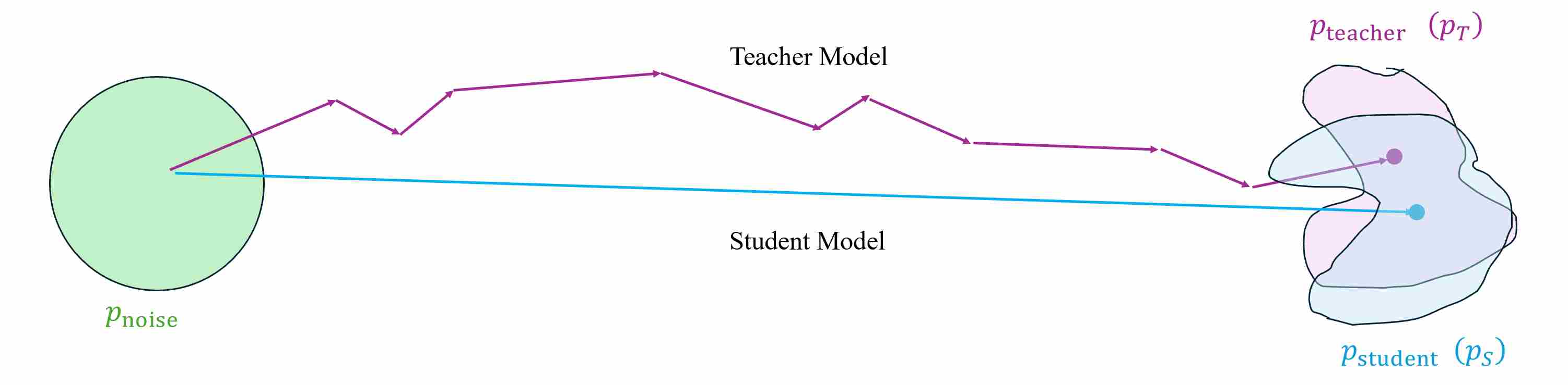
To make it feasible, the DMD design consists of three network structures.
Base (real) denoiser $\mu_{\text{base}}(x_t,t)$: a pretrained diffusion model (EDM or Stable Diffusion) used as a frozen score estimator for the diffused real distribution.
One-step generator $G_\theta(z)$: same architecture as the denoiser but no time input; initialized from the base model’s weights (mean-prediction form in the paper, works identically with $\epsilon$-prediction).
Fake (dynamic) denoiser $\mu_{\phi}^{\text{fake}}(x_t,t)$: trainable denoiser that continuously fits the current student distribution (used to compute the fake score).
10.1.2 Principle and Formulation
Two ingredients make DMD work, The final generator loss consists of two components
Distribution-Matching Loss. which is used to minimize the student output distribution ($p_{\text{fake}}$) and the teacher output distribution ($p_{\text{real}}$).
\[D_{\mathrm{KL}}\big(p_{\text{fake}}\ \| \ p_{\text{real}}\big)\;=\;\mathbb{E}_{x\sim p_{\text{fake}}}\big[\log p_{\text{fake}}(x)-\log p_{\text{real}}(x)\big],\]Regression Loss. The KL gradient above is well-behaved at moderate–high noise but can get unreliable at very low noise (real density nearly zero off-manifold). Also, scores are invariant to scaling of the density, which can invite mode collapse/dropping. DMD therefore adds a tiny amount of paired supervision: precompute a small set of (noise, multi-step output) pairs $(z,y)$ from the base model via a deterministic ODE sampler, and minimize
\[\mathcal L_{\text{reg}}=\mathbb{E}_{(z,y)}\,\text{LPIPS}\big(G_\theta(z),\,y\big).\]where $\text{LPIPS}$ 15 is an abbreviation for Learned Perceptual Image Patch Similarity, a learned deep feature–based metric that measures perceptual similarity between two images, capturing human visual judgment more accurately than pixel-wise distances or conventional perceptual losses.
The final generator loss is
\[\mathcal L_G=D_{\mathrm{KL}}+\lambda_{\text{reg}}\,\mathcal L_{\text{reg}}\quad (\lambda_{\text{reg}}=0.25 \text{ by default}).\]The following figure shows optimizing various objectives starting from the initial state leads to different outcomes.
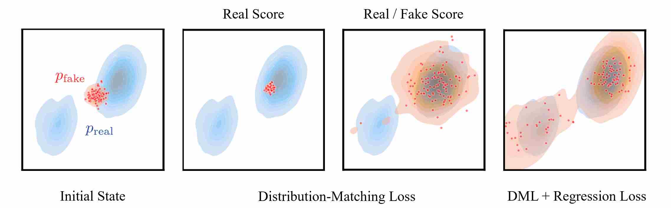
10.1.3 The core objective: KL Divergence
DMD minimizes
\[D_{\mathrm{KL}}\big(p_{\text{fake}}\ \| \ p_{\text{real}}\big)\;=\;\mathbb{E}_{x\sim p_{\text{fake}}}\big[\log p_{\text{fake}}(x)-\log p_{\text{real}}(x)\big],\]with $x=G_\theta(z),\ z\sim\mathcal N(0,I)$. Differentiating w.r.t. $\theta$ using reparameterization gives
\[\nabla_\theta D_{\mathrm{KL}}\;=\; \mathbb{E}_{z}\Big[\big(s_{\text{fake}}(x)-s_{\text{real}}(x)\big)\,\frac{\partial G_\theta}{\partial\theta}\Big],\]where $s(\cdot)=\nabla_x \log p(\cdot)$ is the score. Intuition: $s_{\text{real}}$ pushes samples toward real modes; $-s_{\text{fake}}$ “spreads” samples away from spurious fake modes. The generator update thus follows (fake − real).
However, two issues arise in the image space:
Scores may be undefined where the other distribution has zero density, that’s because at the very beginning, there is almost no overlap between $p_{\text{fake}}$ and $p_{\text{real}}$, according to the score definition
\[s_{\text{real}} = \nabla_x \log p_{\text{real}}(x) = \frac{\nabla_x p_{\text{real}}(x)}{p_{\text{real}}(x)}\]since $x\sim p_{\text{fake}}$, makes $p_{\text{real}}(x) = 0$ for most area.
We don’t know the exact distribution of $p_{\text{real}}$ and $p_{\text{fake}}$.
Diffusion models estimate conditional scores, not the marginal data distribution. The fix is to work in diffusion space: perturb $x$ with Gaussian noise to obtain
\[x_t\sim q_t(x_t \mid x)=\mathcal N(\alpha_t x,\sigma_t^2 I),\]where supports overlap and denoisers approximate the corresponding scores.
Using mean-prediction form 3, the scores at time $t$ are
\[s_{\text{real}}(x_t,t)= -\frac{x_t-\alpha_t\,\mu_{\theta}^{\text{real}}(x_t,t)}{\sigma_t^2},\qquad s_{\text{fake}}(x_t,t)= -\frac{x_t-\alpha_t\,\mu_{\phi}^{\text{fake}}(x_t,t)}{\sigma_t^2}.\]Then the distribution-matching update becomes
\[\nabla_\theta D_{\mathrm{KL}} \;\approx\; \mathbb{E}_{z,t,x,x_t}\left[ w_t\,\alpha_t\,\big(s_{\text{fake}}(x_t,t)-s_{\text{real}}(x_t,t)\big)\,\frac{\mathrm d G}{\mathrm d\theta} \right],\]with a carefully chosen time weight $w_t$ to normalize gradient magnitudes across noise levels.
10.1.4 How the "fake denoiser" is trained
Because the student’s output distribution keeps evolving, DMD trains a dynamic fake denoiser \(\mu_{\phi}^{\text{fake}}\) to track the current fake distribution. Training uses a standard diffusion denoising loss
\[\mathcal L_{\text{denoise}}(\phi) = \big\|\mu_{\phi}^{\text{fake}}(x_t,t)-x_0\big\|_2^2,\]where $x_0$ is the (stop-grad) student output that was just diffused to form $x_t$. This keeps $\mu_{\phi}^{\text{fake}}$ on-support for the fake distribution, so its score is numerically stable and informative for the generator update.
Interpretation: Functionally, $\mu_{\phi}^{\text{fake}}$ serves as a pseudo-teacher in diffusion space for the student’s current distribution, while the frozen base $\mu_{\text{base}}$ provides the real score. The generator’s gradient is driven by the difference of the two. Data-flow wise, though, $G_\theta$ supplies the data to train $\mu_{\phi}^{\text{fake}}$, creating a bootstrapped self-distillation loop.
10.1.5 A Canonical Training Algorithm (Template)
Below is a minimal, implementation-oriented template that captures the core algorithmic skeleton independent of specific papers.
# Distribution Matching Distillation (DMD)

# Inputs:
#   G_theta: The one-step student generator
#   mu_base: Frozen base diffusion model (Real Score Estimator)
#   mu_fake: Trainable diffusion model (Fake Score Estimator)

for each training step:
    # --- 1. Train the Fake Denoiser (mu_fake) ---
    # Generate data from current student (without gradients for this part)
    z ~ N(0, I)
    with no_grad:
        x_fake = G_theta(z)

    # Standard diffusion training on generated data
    t ~ Uniform(0, T)
    eps ~ N(0, I)
    x_t = diffuse(x_fake, t, eps)

    loss_denoiser = MSE(mu_fake(x_t, t), x_fake)
    update(mu_fake, loss_denoiser)

    # --- 2. Train the Generator (G_theta) ---
    # Now we need gradients through G
    z ~ N(0, I)
    x_gen = G_theta(z)

    # Sample time for score matching
    t ~ Uniform(0, T)
    eps ~ N(0, I)
    x_t_gen = diffuse(x_gen, t, eps)

    # Compute Scores (via epsilon prediction or mu prediction)
    with no_grad:
        # Real score direction (where real data is)
        score_real = (x_t_gen - alpha[t]*mu_base(x_t_gen, t)) / sigma[t]^2

        # Fake score direction (where current student data is)
        # Note: mu_fake is kept current by step 1
        score_fake = (x_t_gen - alpha[t]*mu_fake(x_t_gen, t)) / sigma[t]^2

    # The Gradient Update Rule:
    # grad_G ~ (score_fake - score_real) * dG/dtheta
    # We implement this via a "surrogate loss" whose gradient matches the above

    # L_KL = D_KL(p_fake || p_real)
    # We treat (score_real - score_fake) as a fixed weight vector for x_gen
    grad_weight = score_real - score_fake

    # Backward pass trick: dot product
    L_approx = dot_product(x_gen, grad_weight.detach())

    # Add Regression Loss (LPIPS) on paired data to prevent mode collapse
    L_reg = LPIPS(x_gen, precomputed_teacher_trajectory(z))

    # Minimize L_approx (maximizes likelihood) + minimize L_reg
    # Note: Since we defined grad_weight = real - fake, maximizing dot product
    # moves x_gen towards real and away from fake.
    # So we minimize: -L_approx
    L_total = -L_approx + lambda * L_reg

    update(G_theta, L_total)
Inference Strategy: DMD transforms the diffusion model into a pure one-step generator. Inference is trivial: you sample Gaussian noise \(z \sim \mathcal{N}(0, I)\) and feed it directly into the generator $G_\theta(z)$. The model outputs the final image $x$ immediately. Because DMD aligns the student’s output distribution with the teacher’s implied distribution (rather than just minimizing per-sample error), the resulting images are sharp and diverse without requiring a scheduler, solver, or any iterative refinement steps.
10.2 Improved Distribution Matching Distillation (DMD2)
DMD2 16 revisits the original DMD pipeline and identifies why DMD needs the paired regression regularizer in practice: the distribution-matching gradient is only as reliable as the two score estimators (real score from the frozen teacher, fake score from the online critic). DMD2 makes four tightly coupled changes:
- Remove the regression loss (and thus the expensive noise–image pair dataset). This removes an implicit “upper bound” that ties the student to the teacher’s deterministic sampling paths.
- Stabilize “pure distribution matching” by a Two Time-scale Update Rule (TTUR): update the fake score model more frequently than the generator.
- Add a GAN term trained on real data, so the student can correct teacher-score approximation errors and potentially surpass the teacher.
- Support multi-step generation, and fix the training–inference mismatch via backward simulation: train using intermediate inputs produced by the current student (not by forward-diffusing real images).
10.2.2 The core objective (I): Pure distribution matching, without regression pairs
Recall DMD’s distribution-level target: match the diffused student distribution \(p_{\text{fake},t}\) to the diffused target (teacher/data) distribution \(p_{\text{real},t}\) across noise levels.
Let the forward diffusion (noise injection) be
\[x_t = F(x,t)=\alpha_t x + \sigma_t \epsilon,\qquad \epsilon\sim\mathcal N(0,I).\]A diffusion denoiser \(\mu(x_t,t)\) induces a score estimator for the diffused marginal via the standard identity:
\[s(x_t,t)=\nabla_{x_t}\log p_t(x_t) = -\frac{x_t-\alpha_t\,\mu(x_t,t)}{\sigma_t^2}.\]DMD parameterizes two scores:
- Real score \(s_{\text{real}}(x_t,t)\) from a frozen teacher diffusion model \(\mu_{\text{real}}\).
- Fake score \(s_{\text{fake}}(x_t,t)\) from an online diffusion critic \(\mu_{\text{fake}}\) trained on samples from the current generator.
For a one-step generator \(x=G_\theta(z),\ z\sim\mathcal N(0,I)\), DMD only needs the gradient of the expected KL:
\[\mathcal L_{\text{DMD}}(\theta)=\mathbb E_t\Big[ D_{\mathrm{KL}}(p_{\text{fake},t}\ \|\ p_{\text{real},t})\Big].\]The key score-difference gradient used to update \(G_\theta\) is:
\[\nabla_\theta \mathcal L_{\text{DMD}} = -\mathbb E_{t,z,\epsilon}\Big[ \Big( s_{\text{real}}\big(F(G_\theta(z),t),t\big) - s_{\text{fake}}\big(F(G_\theta(z),t),t\big) \Big)^\top \frac{\partial G_\theta(z)}{\partial\theta} \Big].\]DMD2 keeps this distribution matching objective, but drops the paired regression term. In DMD, a regression regularizer was added:
\[\mathcal L_{\text{reg}}=\mathbb E_{(z,y)}\, d\big(G_\theta(z),y\big),\]where \(y\) is a teacher-generated image from a deterministic sampler given the same noise \(z\). This is precisely the part DMD2 removes to eliminate dataset construction and to avoid anchoring the student to teacher sampling trajectories.
So, at this stage, DMD2’s generator is trained by pure distribution matching without \(\mathcal L_{\text{reg}}\).
\[\min_\theta\ \mathcal L_{\text{DMD}}(\theta),\]10.2.3 The core objective (II): Stabilize with Two Time-scale Update Rule (TTUR)
Naively removing \(\mathcal L_{\text{reg}}\) makes training unstable: the culprit is \(\mu_{\text{fake}}\) lagging behind the rapidly changing generator distribution, which biases the score-difference gradient.
DMD2’s fix is TTUR: train \(\mu_{\text{fake}}\) at a higher frequency than the generator so that the fake score tracks the generator’s current output distribution more accurately. Concretely, the paper uses: 5 fake score updates per 1 generator update.
This single scheduling change is enough to make “pure distribution matching” stable and competitive, without any regression pairs.
10.2.4 The core objective (III): Add a GAN loss trained on real images
Even with TTUR, DMD2 observes a residual quality gap vs the teacher. The paper hypothesizes a fundamental reason:
- The “real score” \(\mu_{\text{real}}\) is itself an approximation, so its error propagates through the distribution matching gradient.
- DMD-style training never directly uses real images, so it cannot correct these teacher-score errors.
DMD2 addresses this by adding a GAN objective with real data. The discriminator is implemented as a classification branch attached to the bottleneck of the fake diffusion denoiser (a minimalist “diffusion-as-discriminator” design).
The GAN is applied in diffusion space: discriminate between noised real images \(F(x,t)\) and noised generated images \(F(G_\theta(z),t)\). The paper writes the standard non-saturating objective:
\[\mathcal L_{\text{GAN}} = \mathbb E_{x\sim p_{\text{real}},\,t}\big[\log D(F(x,t))\big] + \mathbb E_{z\sim\mathcal N(0,I),\,t}\big[-\log D(F(G_\theta(z),t))\big].\]Operationally, one can view this as:
Discriminator (maximize real / minimize fake):
\[\max_D\ \mathbb E_{x,t}\big[\log D(F(x,t))\big] + \mathbb E_{z,t}\big[\log(1-D(F(G_\theta(z),t)))\big].\]Generator (fool discriminator):
\[\min_\theta\ \mathcal L_G^{\text{GAN}} = \mathbb E_{z,t}\big[-\log D(F(G_\theta(z),t))\big].\]
Finally, DMD2 updates \(G_\theta\) using both:
- the implicit distribution matching gradient (score difference),
- and the explicit GAN generator loss \(\mathcal L_G^{\text{GAN}}\).
10.2.5 Few-step extension: denoise–re-noise sampling, and backward simulation
For large-scale models (e.g., SDXL), the paper finds one-step mapping “noise → highly diverse images” too hard, and extends the student to a few-step generator with a fixed schedule shared by training and inference.
Inference (N-step). Fix a timestep schedule \(\{t_1,t_2,\ldots,t_N\}\) (paper example for a 1000-step teacher: \(999,749,499,249\)). Starting from pure noise \(z_0\sim\mathcal N(0,I)\), alternate:
Denoise (student step):
\[\hat x_{t_i} = G_\theta(x_{t_i},t_i),\]Re-noise (forward diffusion):
\[x_{t_{i+1}} = \alpha_{t_{i+1}}\hat x_{t_i}+\sigma_{t_{i+1}}\epsilon,\qquad \epsilon\sim\mathcal N(0,I),\]
until the final image \(\hat x_{t_N}\) is produced. This “denoise–re-noise” loop is explicitly inspired by the sampling style of consistency models, but here the step operator is learned by distribution matching + GAN.
Training–inference mismatch. A common pitfall for multi-step generators is: training uses forward-diffused real images as inputs, but inference uses intermediate states coming from previous student steps. DMD2 fixes this by backward simulation:
- During training, instead of feeding \(G_\theta\) with \(F(x_{\text{real}},t_i)\), we generate intermediate noisy states \(x_{t_i}\) by running the current student for a few steps (same pipeline as inference).
- Then we supervise the student outputs using the same proposed losses (distribution matching gradient + GAN), now under the correct input distribution.
This closes the train/test gap while remaining practical because the student only runs for a few steps.
10.2.6 A Canonical Training Algorithm (DMD2 Pseudocode)
Below is a minimal, implementation-oriented template that captures the core algorithmic skeleton independent of specific papers.
# DMD2: Improved Distribution Matching Distillation
#
# Components:
#   mu_real: frozen teacher diffusion model (real score estimator)
#   mu_fake: trainable diffusion model (fake score estimator)
#   D:       classifier branch on mu_fake bottleneck (GAN discriminator)
#   G_theta: student generator (one-step: x = G(z); few-step: x_hat = G(x_t, t))
#
# Hyper-params:
#   K = 5          # TTUR: fake score updates per generator update
#   lambda_gan     # GAN weight
#   schedule = [t1, ..., tN]  # N-step schedule (N=1 reduces to one-step)

for each training iteration:

    # -----------------------------
    # (A) Backward simulation (for N-step training)
    # -----------------------------
    z0 ~ N(0, I)
    x_t = z0
    xt_list = []
    for i in range(N):
        xt_list.append( (x_t, schedule[i]) )
        with no_grad:
            x_hat = G_theta(x_t, schedule[i])         # denoise
        if i < N-1:
            eps ~ N(0, I)
            x_t = alpha[schedule[i+1]] * x_hat + sigma[schedule[i+1]] * eps  # re-noise

    # final generated image (used for GAN + optional logging)
    x_gen = x_hat

    # -----------------------------
    # (B) Update mu_fake (+ discriminator) with higher frequency (TTUR)
    # -----------------------------
    for k in range(K):
        # 1) train fake diffusion score model mu_fake on generated samples
        t ~ Uniform(0, T)
        eps ~ N(0, I)
        x_t_fake = diffuse(x_gen, t, eps)
        loss_fake_score = MSE(mu_fake(x_t_fake, t), x_gen)   # mean-prediction form (consistent with the paper)
        update(mu_fake, loss_fake_score)

        # 2) train discriminator D using real images + generated images (both noised)
        x_real ~ dataset_batch()
        t ~ Uniform(0, T)
        eps_r, eps_f ~ N(0, I), N(0, I)
        x_r_t = diffuse(x_real, t, eps_r)
        x_f_t = diffuse(x_gen.detach(), t, eps_f)

        # non-saturating GAN discriminator objective
        loss_D = -log(D(x_r_t, t)) - log(1 - D(x_f_t, t))
        update(D, loss_D)   # (in practice D shares encoder with mu_fake bottleneck)

    # -----------------------------
    # (C) Update generator G_theta: distribution matching gradient + GAN loss
    # -----------------------------
    # (optionally) sum over steps; here we show a step-summed version
    L_dm = 0
    for (x_in, t_in) in xt_list:
        x_hat = G_theta(x_in, t_in)        # now WITH gradients

        # compute score difference at a randomly sampled diffusion time
        t ~ Uniform(0, T)
        eps ~ N(0, I)
        x_hat_t = diffuse(x_hat, t, eps)

        with no_grad:
            # scores from denoisers (converted via the standard diffusion-score identity)
            s_real = score_from_denoiser(mu_real, x_hat_t, t)
            s_fake = score_from_denoiser(mu_fake, x_hat_t, t)

        # surrogate loss whose gradient equals the implicit KL gradient in the paper
        # (matches:  ∇θ L_DMD = -(s_real - s_fake)^T * dG/dθ )
        L_dm += - dot(x_hat, (s_real - s_fake).detach())

    # GAN generator loss on real-data discriminator (also in diffusion space)
    t ~ Uniform(0, T)
    eps ~ N(0, I)
    x_gen_t = diffuse(x_gen, t, eps)
    L_gan = -log(D(x_gen_t, t))

    L_total = L_dm + lambda_gan * L_gan
    update(G_theta, L_total)
10.3 f-distill: Generalizing DMD/DMD2 from reverse-KL to f-divergences
Context. In Sec. 10.1–10.2 we saw that DMD/DMD2 essentially optimize a distribution matching objective in diffusion space, where the generator update is driven by a score difference (real/teacher score vs. fake/critic score). DMD corresponds to minimizing a specific f-divergence—reverse KL—and DMD2 adds practical stabilizers (TTUR, GAN term, backward simulation) to make “pure distribution matching” workable in large-scale settings. f-distill 17 extends this line by showing:
- the reverse-KL gradient used by DMD is a special case of a much broader f-divergence family, and
- once generalized, the gradient acquires an explicit density-ratio weighting \(h(r)\) (a function of \(r=p/q\)), which introduces new failure modes: variance blow-up, saturation, and mode dropping/collapse, requiring new stabilization strategies (ratio clipping + two-stage normalization + adversarial ratio estimation).
10.3.1 Setup: intermediate (noised) distributions and f-divergence
Let the teacher induce a (fixed) intermediate/noised distribution \(p_t(x)\) at time \(t\), and the student generator \(G_\theta\) induce \(q_t(x)\). In diffusion distillation we sample:
\[x = G_\theta(z) + \sigma(t)\,\epsilon,\qquad z\sim p(z),\ \epsilon\sim\mathcal N(0,I),\]so \(q_t\) is the distribution of that random variable. Define the f-divergence between teacher distribution and student distribution:
\[D_f(p_t \| q_t)\;=\;\int q_t(x)\, f\!\Big(\frac{p_t(x)}{q_t(x)}\Big)\,dx,\]with \(f\) convex and \(f(1)=0\).
10.3.2 Step-by-step derivation
Represented the ratio \(p_t/q_t\) as \(r_t\), Differentiate the integrand
\[\small \begin{align} \nabla_\theta D_f(p_t \|q_t) & =\nabla_\theta \int q_t(x)\, f\!\Big(\frac{p_t(x)}{q_t(x)}\Big)\,dx = \nabla_\theta \int q_t(x)\,f\Big(r_t(x)\Big)\,dx \\[10pt] & = \int \nabla_\theta q_t(x)\, f\!\Big(r_t(x)\Big)\,dx \;+\;\int q_t(x)\,\nabla_\theta f\!\Big(r_t(x)\Big)\,dx \\[10pt] & = \int \nabla_\theta q_t(x)\, f\!\Big(r_t(x)\Big)\,dx \;+\;\int q_t(x)\, f^{'}\!\Big(r_t(x)\Big) \nabla_\theta r_t(x)\,dx \\[10pt] & = \int \nabla_\theta q_t(x)\, f\!\Big(r_t(x)\Big)\,dx \;+\;\int q_t(x)\, f^{'}\!\Big(r_t(x)\Big) \Big(-\frac{p_t(x)\nabla_{\theta} q_t(x)}{q_t^2(x)}\Big)\,dx \\[10pt] & = \underbrace{\int \nabla_\theta q_t(x)\, f\!\Big(r_t(x)\Big)\,dx}_{I} \;+\;\underbrace{\int \nabla_\theta q_t(x)\, \Big(-r_t(x)\, f^{'}\!\Big(r_t(x)\Big)\Big)\,dx}_{II} \end{align}\]Both \(I\) and \(II\) are of the form
\[\int \nabla_\theta q_t(x)\, g(x)\,dx,\]where \(g(x)=f\!(r_t(x))\) in $I$, and \(g(x)=-r_t(x)\, f^{'}\!(r_t(x))\) in $II$. Assuming that sampling from \(x \sim q_t(x)\) can be parameterized to \(x = G_{\theta}(z) + \sigma(t)\epsilon\) with \(z \sim p(z)\), and \(\epsilon \sim \mathcal N(0, I)\) and \(G_\theta,\, g\) are differentiable mappings. In addition, \(g\) is constant with respect to $\theta$.
\[\begin{align} \int (\nabla_\theta q_t(x))\,g(x)\,dx & = \nabla_\theta \int ( q_t(x))\,g(x)\,dx \\[10pt] & = \nabla_\theta \int \int p(z)\,p(\epsilon)\,g(G_\theta(z)+\sigma(t)\epsilon)\,d\epsilon\,dz \\[10pt] & = \int \int p(z)\,p(\epsilon)\,\nabla_\theta g(G_\theta(z)+\sigma(t)\epsilon)\,d\epsilon\,dz \\[10pt] & = \int \int p(z)\,p(\epsilon)\,\nabla_x g(x)\,\nabla_\theta G_\theta\,d\epsilon\,dz \end{align}\]compute \(\nabla_x g(x)\) for (I) and (II). For (I):
\[\nabla_x g(x) = \nabla_x f(r_t(x)) = f^{'}(r_t(x))\,{r_t}^{'}(x). \label{eq:I}\]and For (II):
\[\small \nabla_x g(x) = \nabla_x \Big(f^{'}(r_t(x))\,r_t(x) \Big)= f^{''}(r_t(x))\,{r_t}^{'}(x)\,r_t(x)+f^{'}(r_t(x))\,{r_t}^{'}(x). \label{eq:II}\]Substitute Eq. \ref{eq:I} and Eq. \ref{eq:II} into \(\nabla_\theta D_f(p_t \|q_t)\), and simplify to obtain
\[\small \begin{align} \nabla_\theta D_f(p_t \|q_t) & = \mathbb E_{z,\epsilon} \Big[\nabla_x f(r_t(x))\,\nabla_\theta G_\theta\Big] \;-\; \mathbb E_{z,\epsilon} \Big[\nabla_x \Big(f^{'}(r_t(x))\,r_t(x) \Big)\,\nabla_\theta G_\theta\Big] \\[10pt] & = \mathbb E_{z,\epsilon} \Big[ \Big(\nabla_x f(r_t(x)) - \nabla_x \Big(f^{'}(r_t(x))\,r_t(x) \Big)\Big)\,\nabla_\theta G_\theta \Big] \\[10pt] & = \mathbb E_{z,\epsilon} \Big[ \Big(f^{'}(r_t(x))\,{r_t}^{'}(x) - f^{''}(r_t(x))\,{r_t}^{'}(x)\,r_t(x)+f^{'}(r_t(x))\,{r_t}^{'}(x)\Big)\,\nabla_\theta G_\theta\Big]\\[10pt] & = - \mathbb E_{z,\epsilon} \Big[ \Big(f^{''}(r_t(x))\,{r_t}^{'}(x)\,r_t(x)\Big)\,\nabla_\theta G_\theta \Big] \\[10pt] & = - \mathbb E_{z,\epsilon} \Big[ \Big(f^{''}(r_t(x))\,r_t^2(x)\,\nabla_x \log {r_t}(x)\Big)\,\nabla_\theta G_\theta \Big] \\[10pt] & = - \mathbb E_{z,\epsilon} \Big[f^{''}(r_t(x))\,r_t^2(x)\,\Big(\,\underbrace{\nabla_x \log p_t(x)}_{\text{teacher score}} - \underbrace{\nabla_x \log q_t(x)}_{\text{fake score}}\,\Big)\,\nabla_\theta G_\theta\Big] \end{align}\]In practice, we minimize the f-divergence along the whole time range, i.e.,
\[\mathcal L(\theta) = \int_0^T w_t D_f(p_t \|q_t) dt\]where $w_t$ is a time-dependent weight for equalizing the gradient magnitudes across times. To implement this without backpropagating through the score networks (and to keep it aligned with DMD/DMD2 practice), f-distill uses a stop-gradient surrogate objective:
\[\mathcal{L}_{f\text{-distill}}(\theta) = \mathbb{E}_{t,x}\Big[ \mathrm{sg}\Big(w_t\, h(r_t(x))\big(\nabla_x\log p_t(x)-\nabla_x\log q_t(x)\big)\Big)^\top x\Big],\]where
\[h(r_t(x))= f^{''}(r_t(x))\,r_t^2(x)\]and \(x=G_\theta(z)+\sigma(t)\epsilon\) and \(\mathrm{sg}(\cdot)\) is stop-gradient.
10.3.3 Practical instantiation in diffusion distillation: estimating the density ratio as a literal fraction
The theorem introduces \(r_t(x)=p_t(x)/q_t(x)\), which is not directly accessible. f-distill estimates it adversarially, using a GAN-style discriminator in diffusion space.
A standard result: if \(D_\lambda(x_t,t)\) is trained to output the probability that a sample at time $t$ is real (from \(p_{data,t}\)) vs fake (from \(q_t\)), then the optimal discriminator satisfies:
\[D^*(x)=\frac{p(x)}{p(x)+q(x)} \quad\Rightarrow\quad \frac{p(x)}{q(x)}=\frac{D^*(x)}{1-D^*(x)}.\]The paper explicitly uses this fraction form:
\[r(x_t)=\frac{p_t(x)}{q_t(x)}\approx \frac{D_\lambda(x_t,t)}{1-D_\lambda(x_t,t)}.\]Depending on implementation, you may parameterize the discriminator as a logit approximating \(\log r\), in which case \(r=\exp(\text{logit})\)
10.3.4 What new problems appear and Stabilization strategies
Once we move away from reverse-KL, the update becomes:
\[\text{(weight)}\times\text{(score difference)}.\]This is powerful (you can tune mode-coverage/diversity trade-offs), but it introduces three engineering-critical instabilities:
Mode-seeking / diversity drop: Different f-divergences have different mode-seeking tendencies. The paper highlights that reverse-KL is mode-seeking, and discusses criteria (e.g., behavior of \(\lim_{r\to\infty} f(r)/r\)) showing reverse-KL and JS have finite limits (mode-seeking), while forward-KL has an infinite limit (mode-covering).
It also connects mode-seeking behavior to the growth of \(h(r)\): divergences that are less mode-seeking tend to have a weighting \(h(r)\) that increases more strongly with large $r$, putting more pressure on regions where the teacher assigns higher density relative to the student.
Saturation (vanishing gradients when \(r\) is extreme): Early training often yields very poor alignment, so \(r=p/q\) becomes either huge or near zero. For some divergences (e.g., JS, squared Hellinger), gradients become small at both extremes → saturation and slow/unstable optimization.
High variance from ratio-weighting \(h(r)\): Even if the expectation is correct, the variance of \(h(r)\) can explode when distributions are far apart, producing noisy gradients and training collapse. The paper quantifies this using a normalized variance measure and observes large variance growth for some divergences (e.g., forward-KL, Jeffreys) as mismatch increases, while JS and squared Hellinger stay relatively stable.
f-distill’s key message is: a unified objective does not mean a unified training recipe. Once \(h(r)\) enters, you must stabilize the ratio-weighted gradients. The paper proposes (and codifies in Algorithm 1) three practically important techniques:
Density-ratio clipping: Compute \(r\) from the discriminator (either via \(D/(1-D)\) or \(\exp(\log r)\)), then clip:
\[r \leftarrow \mathrm{clip}(r,\ r_{\min},\ r_{\max}).\]This directly combats saturation (extreme $r$) and reduces variance spikes.
Two-stage normalization (the “variance killer”): To handle high-variance weights, the paper proposes two-stage normalization:
Stage 1 (normalize ratios): exploit \(\mathbb E_{q_t}[r_t]=1\) and normalize $r$ (in practice, within time bins / per-batch normalization). Algorithmically: \(\bar r_i = r_i / \sum_i r_i\).
Stage 2 (normalize weights): compute \(h_i=h(\bar r_i)\), then normalize to keep mean weight ~ 1:
The paper motivates this normalization explicitly as the remedy for high variance in $h$.
Keep the DMD2-style adversarial loop (TTUR-like updates + GAN term): Like DMD2, f-distill uses an adversarial training structure:
- update the student \(G_\theta\) less frequently than the critic components (fake score + discriminator),
- and keep an explicit GAN generator loss term in addition to the f-distill gradient.
This is conceptually aligned with DMD2’s “pure distribution matching needs stabilizers”: TTUR and GAN-on-real-data are essential when the distribution-matching gradient relies on learned critics.
11. Score-Based Distillation
Score-based distillation is built on the principle distill the teacher’s score field. While Sec. 10 (“distribution distillation”) emphasizes matching terminal distributions via divergences, score distillation pushes the student using local gradients of log-density—i.e., the score. This is natural because, as established earlier in this post, noise prediction is equivalent to score estimation. In this chapter, we will:
- Abstract a common objective shared by a broad family of score-based distillation methods.
- Provide a canonical training template (pseudo-code).
- Explain where different methods “plug in” and what they modify (design knobs).
- Focus on fast sampling methods (SiD / SIM / SwiftBrush / extensions up to ~2026).
- Contrast score distillation for amortized acceleration vs score distillation for guidance/editing.
11.1 Unifying View: Distill the Score Residual
Let a pretrained diffusion teacher define a conditional noisy marginal \(p_t^{\text{teacher}}(x_t\mid c)\) with score
\[s_t^{\text{teacher}}(x_t,t,c) \;\triangleq\; \nabla_{x_t}\log p_t^{\text{teacher}}(x_t\mid c).\]We train a fast student sampler $G_{\theta}$ (often one-step or few-step) that induces a distribution \(q_\theta(x_0\mid c)\), and its diffused marginal
\[q_{\theta,t}^{\text{student}}(x_t\mid c) \;=\; \int q_\theta(x_0\mid c)\, q(x_t\mid x_0,t)\,dx_0.\]A clean conceptual objective is to minimize a time-averaged divergence between noisy marginals:
\[\min_\theta\;\; \mathbb{E}_{t\sim \rho(t)}\Big[\,\mathcal{D}\big(q_{\theta,t}^{\text{student}}(\cdot\mid c)\;\|\;p_t^{\text{teacher}}(\cdot\mid c)\big)\Big],\]where \(\rho(t)\) is a chosen time sampling distribution and \(\mathcal{D}\) can be a score-based divergence (e.g., Fisher divergence / score matching-type) or a divergence whose gradient can be expressed using scores.
The key shared structure across “score distillation” methods is: The student update is driven by a score residual
\[r(x_t,t,c)\;\approx\; s_{\text{student}}(x_t,t,c)\;-\;s_{\text{teacher}}(x_t,t,c),\]and we backpropagate this residual through the student’s sampling path. So the only real question becomes:
How do we get an estimate of the student score \(s_{\text{student}}\) (or an equivalent baseline), such that the residual is informative and stable?
That is exactly where different score-based distillation algorighms (SiD / SIM / SwiftBrush) differ.
11.2 A Common Objective: Score Divergence (and Why It’s Hard)
A canonical “score-matching” divergence between two noisy marginals is the Fisher divergence:
\[\mathcal{D}_F\big(q_{\theta,t}\,\|\,p_T\big) \;=\; \frac{1}{2}\;\mathbb{E}_{x_t\sim q_{\theta,t}} \left[ \left\| s_{\theta}(x_t,t,c)-s_{\text{teacher}}(x_t,t,c) \right\|^2 \right],\]where
\[s_\theta(x_t,t,c)=\nabla_{x_t}\log q_{\theta,t}^{\text{student}}(x_t\mid c).\]If we could evaluate \(s_\theta\), the problem would reduce to standard score matching. But for a generator-defined (implicit) distribution \(q_\theta\), \(\nabla_{x_t}\log q_{\theta,t}^{\text{student}}\) is typically intractable. This leads to the central technical motif:
- Teacher score \(s_{\text{teacher}}\) is available “for free” from the pretrained diffusion model.
- Student score \(s_\theta\) is not directly available.
- Score distillation methods mainly differ in how they approximate or avoid \(s_\theta\).
The most common solutions are:
Analytic baseline score (from the corruption kernel \(q(x_t\mid x_0,t)\)), which yields SDS-like gradients (guidance-style). Concretly, we use score (Fisher) identity to compute \(s_\theta\)
\[\begin{align} \nabla_{x_t}\log q_{\theta,t}(x_t\mid c) &= \frac{1}{q_{\theta,t}(x_t\mid c)}\nabla_{x_t}\int q_\theta(x_0\mid c)\,q(x_t\mid x_0,t)\,dx_0 \\[10pt] &= \frac{1}{q_{\theta,t}(x_t\mid c)}\int q_\theta(x_0\mid c)\,\nabla_{x_t}q(x_t\mid x_0,t)\,dx_0 \\[10pt] &= \int \underbrace{\frac{q_\theta(x_0\mid c)\,q(x_t\mid x_0,t)}{q_{\theta,t}(x_t\mid c)}}_{q_\theta(x_0\mid x_t,c)} \;\nabla_{x_t}\log q(x_t\mid x_0,t)\,dx_0 \\[10pt] &= \mathbb E_{x_0\sim q_\theta(\cdot\mid x_t,c)}\Big[\nabla_{x_t}\log q(x_t\mid x_0,t)\Big]. \end{align}\]this implies that the student marginal score admits the representation
\[\begin{align} s_\theta(x_t,t,c) & =\nabla_{x_t}\log q_{\theta,t}(x_t\mid c)=\mathbb E_{x_0\sim q_\theta(\cdot\mid x_t,c)}\Big[\nabla_{x_t}\log q(x_t\mid x_0,t)\Big] \\[10pt] & = E_{x_0\sim q_\theta(\cdot\mid x_t,c)}\Big[-\frac{x_t-\alpha_t x_0}{\sigma_t^2}\Big] = \mathbb E\Big[-\frac{\epsilon}{\sigma_t}\ \Big|\ x_t,c\Big]. \end{align}\]In practice, SDE uses a single-sample Monte Carlo baseline
\[s_\theta \triangleq -\frac{\epsilon}{\sigma_t},\]- Learn an auxiliary/online score model to approximate \(s_\theta\) (VSD line; also used by many fast one-step methods).
- Score identities / implicit matching that let you estimate the needed gradient without explicitly computing \(s_\theta\) (SiD / SIM family).
11.3 A Canonical Training Algorithm (Template)
Below is a unified template that captures most practical score-distillation systems for amortized fast sampling.
It separates the method into two conceptual blocks:
- (A) Student sampler: one-step or few-step generator that produces \(x_0\).
- (B) Student-score estimator: either analytic, learned (online diffusion), or identity-based.
The update rule is expressed using the detached score residual to prevent second-order coupling unless explicitly desired.
# ------------------------------------------------------------
# Canonical Score-Based Distillation (Amortized Fast Sampling)
# ------------------------------------------------------------
# Teacher: pretrained diffusion/score model (frozen)
#   - either epsilon-predictor eps_T(xt, t, c)
#   - or denoiser D_T(xt, t, c)
#
# Student: fast sampler producing x0
#   - one-step generator: x0 = G_theta(z, c)
#   - or few-step student with its own internal steps
#
# Optional: online/aux score model approximating student's noisy marginal score
#   - eps_A(xt, t, c) or s_A(xt, t, c)
#
# Goal: minimize a time-averaged score divergence by using a score residual.

for it in range(num_iters):

    # -------------------------
    # 1) sample condition & noise
    # -------------------------
    c   = sample_condition()          # text prompt / class label / etc.
    z   = Normal(0, I).sample()
    t   = sample_time(rho)            # t ~ rho(t)
    eps = Normal(0, I).sample()

    # -------------------------
    # 2) student generates x0 and we diffuse to xt
    # -------------------------
    x0 = G_theta(z, c)                # fast sample (one-step or few-step)
    xt = alpha(t) * x0 + sigma(t) * eps

    # -------------------------
    # 3) teacher score (frozen)
    # -------------------------
    with no_grad():
        eps_T = teacher_eps(xt, t, c)     # or teacher_denoiser(...)
        s_T   = eps_to_score(eps_T, t)    # convert to score if needed

    # -------------------------
    # 4) estimate student score (algorithm-specific)
    # -------------------------
    # (i) analytic baseline: from q(xt|x0,t)  -> SDS-like
    # (ii) learned baseline: s_A = online_score_model(xt,t,c) -> VSD-like
    # (iii) identity / implicit matching -> SiD / SIM-like
    s_hat = estimate_student_score(xt, t, c, x0, eps)  # returns ~ s_theta or a baseline

    # -------------------------
    # 5) detached score residual drives student update
    # -------------------------
    r = (s_hat - s_T).detach()

    # A simple surrogate whose gradient matches "move xt along -r"
    # (many papers use equivalent forms; this one is easy to implement)
    loss_theta = dot(xt, r)           # sum over dimensions then mean over batch
    update(G_theta, loss_theta)

    # -------------------------
    # 6) if using an online score model, train it on student samples
    # -------------------------
    if online_score_model:
        # standard denoising score matching on samples from q_theta
        t2, eps2 = sample_time(rho2), Normal(0,I).sample()
        xt2 = alpha(t2) * x0.detach() + sigma(t2) * eps2
        loss_aux = dsm_loss(online_score_model, xt2, t2, c, eps2)
        update(online_score_model, loss_aux)
This template is intentionally abstract. It captures the dominant “engineering reality” of score distillation:
- A frozen teacher provides \(s_{\text{teacher}}\) (or \(\epsilon_{\text{teacher}}\)).
- Training uses student samples only (often data-free for distilling a pretrained teacher).
- The key is designing \(\widehat{s}_{\text{student}}\) (or a baseline) so that \(r=\widehat{s}_{\text{student}}-s_{\text{teacher}}\) is stable and meaningful.
11.4 Where Methods Differ: A Practical “Knob List”
Most score-based distillation papers can be understood as modifying a small set of knobs:
| Knob | What it changes | Typical effect |
|---|---|---|
| Student form | one-step generator vs few-step sampler | speed–quality frontier |
| Time sampling \(\rho(t)\) | where gradients come from | balances semantics (large t) vs details (small t) |
| Residual definition \(r\) | what “baseline” score is subtracted | stabilizes training / prevents oversaturation |
| How to get \(s_\theta\) | analytic / learned / identity-based | main difference among SiD/SIM/VSD |
| Conditioning & guidance | CFG baked into training or not | alignment and controllability |
| Extra regularizers | perceptual / adversarial / consistency | texture and realism at 1–4 steps |
Keep this table in mind; the next sections are basically “each method picks a point in this design space.”
11.5 Score Distillation for Fast Sampling (Amortized Acceleration)
We now instantiate the template for representative fast sampling methods.
11.5.1 SiD Family: Score Identity Distillation
Score Identity Distillation (SiD) 18 targets a score-based divergence (commonly Fisher divergence) between the student’s noisy marginal and the teacher’s noisy marginal, but crucially uses score identities to make the optimization feasible for implicit student distributions.
How it plugs into the template:
- Student: typically one-step (or few-step) generator.
- Teacher: frozen diffusion model provides \(s_{\text{teacher}}\) (often through \(\epsilon_{\text{teacher}}\)).
- Key modification: the “estimate_student_score” block is implemented via identity-based approximations (instead of explicitly computing \(\nabla \log q_{\theta,t}^{\text{student}}\)).
- Practical emphasis: data-free distillation of a powerful teacher into a fast sampler (e.g., one-step T2I).
A notable extension is Guided SiD / LSG (Long-Short Guidance) 19, which modifies the conditioning/guidance knob: it designs training signals that better match how guidance is used at inference (e.g., CFG-like behavior), improving prompt fidelity without sacrificing one-step speed.
Inference (Fast Generation). After training, generation is trivial: sample \(z\sim\mathcal{N}(0,I)\) and output \(x_0=G_\theta(z,c)\) in one network evaluation (or a small fixed number for few-step variants).
11.5.2 SIM: Score Implicit Matching
Score Implicit Matching (SIM) 20 can be read as a generalization layer over SiD: it studies a broad class of score-based divergences and derives training objectives that avoid requiring direct access to the student score, yielding a unified framework in which SiD appears as a special case.
How it plugs into the template:
- Student: one-step generator (or fast sampler).
- Teacher: frozen diffusion model score \(s_{\text{teacher}}\).
- Key modification: SIM’s \(\mathcal{D}(\cdot\mid \cdot)\) is not restricted to a single squared-score distance; it proposes implicit/identity-based objectives for more general forms (the objective knob is expanded).
- Implementation pattern: many practical SIM-style systems still adopt an online score estimator (aux diffusion) or an equivalent estimator to stabilize training, but the derivation clarifies what objective you are truly optimizing.
Inference (Fast Generation). Same as SiD: one forward pass (or few passes) through the student.
11.5.3 VSD Line: SwiftBrush (One-Step Text-to-Image by Score Distillation)
In practice, the most “plug-and-play” way to implement score distillation for one-step generation is to learn a baseline / auxiliary score model for the student distribution, producing a residual of the form
\[r \;=\; s_{\text{aux}}(x_t,t,c) - s_{\text{teacher}}(x_t,t,c).\]This is the core idea behind Variational Score Distillation (VSD) 21 (popularized in text-to-3D) and its 2D one-step T2I instantiations such as SwiftBrush 22.
How SwiftBrush plugs into the template:
- Student: a one-step text-to-image generator/sampler.
- Teacher: a pretrained diffusion model.
- Key modification: it commits to the “learned baseline” knob:
estimate_student_score(·)is implemented by an auxiliary/online score model trained on student samples (a VSD-style construction). - Why this matters: subtracting an auxiliary score helps reduce the “oversaturation / collapse” behaviors that appear when using raw teacher gradients alone (a known issue in SDS-like objectives). VSD formalizes this as optimizing a variational objective rather than a naive score-pulling rule.
There are also follow-ups (e.g., SwiftBrush v2 23) that further tune the guidance knob (e.g., dynamic negative guidance / CFG variants) to improve text alignment and detail while staying in the one-step regime.
Inference (Fast Generation). One-step generation: \(x_0=G_\theta(z,c)\). No teacher is needed at inference.
11.5.4 Beyond SiD/SIM/SwiftBrush (Up to ~2026): What Else Counts as Score-Based Distillation for Acceleration?
Besides SiD / SIM / SwiftBrush, several acceleration works can be reasonably viewed as “score-based distillation,” because their primary supervision is a teacher score/denoiser and the student is trained via a score residual (possibly combined with other losses):
- Adversarial Score Identity Distillation (SiDA) 24: adds an adversarial component on top of score-identity-style distillation to surpass the teacher faster / improve perceptual sharpness (hybrid knob: residual + adversarial regularization).
- Few-Step Diffusion via SiD 25: extends SiD from strictly one-step to few-step students (student-form knob) to reach a better quality frontier while staying ultra-fast.
- Score Distillation of Flow-Matching Models 26: generalizes the same score-distillation logic beyond diffusion/SDE parameterizations to flow-matching families, showing the “score residual” view is operator-agnostic.
- Domain-specific one-step restorers (e.g., SR / deblurring) that distill pretrained diffusion priors into one-step networks using VSD-like losses (student-form knob applied to inverse problems). A representative example is OSEDiff 27.
- Diffusion → GAN distillation via score distillation (Diff-Instruct line) 28: distill a diffusion teacher into a non-diffusion generator using VSD/IKL-style objectives (student-form knob becomes “GAN generator”).
Remark. Many real systems are hybrids. For example, “Turbo”-style distillation pipelines are often described as combining adversarial training with a score-distillation term; conceptually, the score residual is still the “teacher semantic prior,” while the discriminator acts as a perceptual regularizer.
11.6 Score Distillation for Guidance / Editing (Not Primarily Acceleration)
A second major branch uses “score distillation” not to train a reusable fast sampler, but to optimize an external variable (a NeRF, an image, a latent, a reconstruction, etc.) so that it becomes compatible with a diffusion prior and a condition.
The archetype is Score Distillation Sampling (SDS) 29 (DreamFusion): it uses the teacher’s denoising residual to form a gradient that updates the target representation. VSD 21 improves stability/faithfulness by introducing a learned baseline that approximates the evolving distribution induced by the optimized variable.
For inverse problems / editing, many methods can be interpreted as constructing specialized posterior score residuals:
- Score Distillation via Reparametrized DDIM (often cited as “score distillation inversion” in the literature): uses a reparameterization to make score-distillation gradients better behaved for inversion/editing pipelines.
- DDS (Delta Denoising Score): constructs a difference of denoising scores to isolate an edit direction while preserving identity/content.
- PDS (Posterior Distillation Sampling): forms a posterior-oriented distillation signal (typically “conditional minus unconditional / prior”) to guide edits under probabilistic framing.
- Stable Score Distillation (SSD) and related variants: focus on stabilizing score-distillation-based optimization for editing tasks.
A canonical guidance-style template (contrast with Sec. 11.3) is:
# ------------------------------------------------------------
# Canonical Score Distillation (Guidance / Editing)
# ------------------------------------------------------------
# Optimize an instance-specific variable w (e.g., NeRF params, image latent, etc.)
# No "student sampler" is learned for general reuse.

for it in range(num_iters):

    t, eps = sample_time(rho), Normal(0,I).sample()

    x0 = render_or_decode(w)                  # current candidate
    xt = alpha(t) * x0 + sigma(t) * eps

    with no_grad():
        eps_T = teacher_eps(xt, t, c)         # conditional teacher
        # sometimes also eps_uncond for CFG-like residuals

    # SDS/VSD-style residual defines gradient direction for w through x0
    residual = build_residual(eps_T, eps, baseline_or_aux, t).detach()

    loss = dot(x0, residual)                  # simple surrogate
    update(w, loss)
The key point: here we are not compressing sampling into a student model; we are solving one instance by iteratively optimizing \(w\).
11.7 Acceleration vs Guidance: Common Core, Different Endgame
We can now cleanly state what is shared and what is different.
11.7.1 Common Core
Both directions rely on the same invariant:
- A pretrained diffusion model provides a local descent direction on an implicit energy landscape via a score (or denoising residual).
- The optimization signal is a score residual (teacher score minus some baseline/aux score).
So at a high level, both can be summarized as: Use teacher scores as gradients to push samples/parameters toward high-density regions.
This is why the same mathematics (score identities, residual baselines, time weighting) reappears across SDS/VSD (guidance) and SiD/SIM/SwiftBrush (distillation for fast sampling).
11.7.2 Key Differences
Optimization target
- Acceleration: optimize model parameters \(\theta\) once; reuse forever.
- Guidance/editing: optimize an instance variable \(w\) per input/prompt.
Goal
- Acceleration: approximate the teacher’s sampling distribution with a fast sampler.
- Guidance/editing: approximate a posterior / constraint-satisfying solution for one instance.
Stability & collapse modes
- Acceleration must preserve global diversity across prompts; collapse is fatal.
- Guidance/editing may tolerate mode preference if it achieves the edit/constraint; stability focuses on identity preservation and avoiding artifacts.
Baselines are more critical in guidance Guidance-style SDS is notorious for oversaturation / over-optimization; VSD-like baselines are often essential. In acceleration, baselines are also important, but the additional degrees of freedom (training distributions, curricula, regularizers) provide more levers.
11.7.3 A Useful Mental Model
- Guidance/editing = online optimization using teacher scores as gradients.
- Acceleration distillation = amortize that optimization into a network, so that the “solution” appears in one/few forward passes.
This “amortization view” is often the most intuitive bridge between the two worlds.
12. Consistency-Based Distillation
Consistency distillation is a path-invariance distillation paradigm: it compresses a long-horizon iterative generation (or inference) procedure into a one-step or few-step mapping by enforcing that predictions made at different time/noise levels—as long as they lie on the same underlying trajectory—must agree in a canonical prediction space.
While “Consistency Models” popularized a particular instantiation, the principle is much broader and applies to diffusion sampling, score/SDE solvers, flow-matching ODEs, annealed MCMC/Langevin dynamics, and more generally any process that evolves a state along a continuous (or discretized) notion of time, noise level, or temperature.
12.1 Core Ingredients of Consistency Distillation
A generic consistency-distillation system can be decomposed into four ingredients.
A canonical prediction space ($\mathcal{Y}$). Choose a representation that encodes the “denoised meaning” of a noisy state.
A known re-noising / transport operator (\(\mathcal R_{t\to s}(x_t;\hat x_0)\)). Given a canonical prediction (e.g., $\hat x_0$) we can deterministically “move” along time by reparameterization.
For example, VP defines the deterministic re-noise map (DDIM-style, $\eta=0$):
\[\mathcal R_{t\to s}(x_t;\hat x_0) = \sqrt{\alpha_s}\,\hat x_0 + \sqrt{1-\alpha_s}\,\hat\epsilon, \quad \hat\epsilon = \frac{x_t-\sqrt{\alpha_t}\,\hat x_0}{\sqrt{1-\alpha_t}}.\]This operator is the bridge that allows comparing predictions at different noise levels.
A teacher signal (explicit or implicit). Consistency distillation needs a reference to avoid collapse:
- Explicit teacher: a pretrained diffusion model / sampler provides $\hat x_0^{\mathrm T}(x_t,t,c)$ or one-step transitions.
- Implicit teacher: an EMA copy of the student acts as a “slow-moving target network” (bootstrapping).
An anti-collapse anchor (boundary condition). Pure self-consistency admits the trivial constant solution. A boundary/identity condition fixes this:
\[f_\theta(x_\epsilon, t_\epsilon, c) \approx x_\epsilon, \qquad t_\epsilon \to 0,\]or more generally: the prediction must match ground-truth (when available) or a trusted teacher target near the endpoint.
12.2 Canonical Prediction Space and the Consistency Constraint
Let $x_t$ denote the state at time/noise level $t$. Consistency distillation trains a student predictor
\[f_\theta:\ (x,t,c)\mapsto y \in \mathcal{Y},\]where \(\mathcal{Y}\) is a canonical prediction space chosen so that all points on the same trajectory should map to the same canonical output. Common choices of \(\mathcal{Y}\) include:
- Clean sample space: \(y=\hat{x}_0\), most common in diffusion-style settings.
- Noise / score / velocity spaces: \(y=\hat\epsilon\), or \(y={\nabla_x \log p_t(x)}\), or \(y=\hat v\).
- Jump/flow-map space: \(y=\hat x_s\), a direct prediction of a later state.
- Latent canonical representations: any “equivalence-class representative” that remains stable along the path
The fundamental consistency condition is: if $x_t$ and $x_s$ lie on the same trajectory (with shared randomness coupling), then
\[f_\theta(x_t,t,c)\ \approx\ f_\theta(x_s,s,c),\qquad t>s.\]Intuitively, the student is trained to output a time-invariant “answer” for every point along a trajectory—so that denoising at different noise levels becomes mutually consistent after accounting for the process dynamics.
12.3 The Generic Objective: Pairwise Time-Consistency
Let \(t > s\) be two noise levels (or continuous times). The central constraint is: The canonical prediction produced at time $t$ should match the canonical prediction produced at time $s$ after transporting the state from $t$ to $s$ using the known dynamics.
A widely used template is a teacher-student / stop-grad form:
\[\mathcal L_{\text{cons}} = \mathbb E_{x_t,\,t>s}\Big[ d\Big( f_\theta(x_t,t,c),\; \underbrace{f_{\theta^-}(x_s,s,c)}_{\text{stop-grad target}} \Big) \Big],\]where $d(\cdot,\cdot)$ is an L2/L1/LPIPS-like metric, and
\[x_s = \mathcal R_{t\to s}\!\big(x_t;\; \hat x_0^{\mathrm{ref}}\big).\]The only remaining design choice is: what is the reference $\hat x_0^{\mathrm{ref}}$ used to build $x_s$?
Two dominant patterns cover most practical systems:
12.3.1 Teacher-Driven Consistency (Distill a Strong Base Model)
Use a strong pretrained teacher to define the reference denoising meaning:
\[\hat x_0^{\mathrm{ref}} = \hat x_0^{\mathrm T}(x_t,t,c).\]Then construct the transported state: \(x_s = \mathcal R_{t\to s}\!\big(x_t;\hat x_0^{\mathrm T}(x_t,t,c)\big).\)
The student is trained so that its prediction at $(x_t,t)$ agrees with a target prediction at $(x_s,s)$ (often from EMA-student or teacher):
\[\mathcal L_{\text{cons}} = \mathbb E\Big[ d\Big( f_\theta(x_t,t,c),\; f_{\theta^-}(x_s,s,c) \Big) \Big].\]12.3.2 Self-Teacher Consistency (EMA Bootstrapping)
When an explicit teacher is unavailable or too expensive, use an EMA target network to define the reference:
\[\hat x_0^{\mathrm{ref}} = f_{\theta^-}(x_t,t,c), \qquad x_s = \mathcal R_{t\to s}(x_t;\hat x_0^{\mathrm{ref}}).\]Then enforce
\[f_\theta(x_t,t,c) \approx f_{\theta^-}(x_s,s,c).\]This turns consistency distillation into a bootstrapped contraction-learning problem: the EMA provides stability, while the boundary condition prevents collapse.
12.4 Boundary and Anchor Conditions
A pure invariance constraint admits degenerate solutions (e.g., constant outputs). In practice, consistency distillation is paired with boundary/anchor constraints that pin the canonical space to a meaningful target. Typical anchors include:
- Data boundary: enforce \(f_\theta(x_0,0)\approx x_0\) (or an equivalent small-noise condition)
- Teacher boundary: align the student’s canonical prediction with a teacher’s high-quality estimate at some reference time
- Reconstruction/likelihood-related constraints: depending on the process, add auxiliary losses that prevent collapse and preserve fidelity
Conceptually, the anchor defines what the invariant quantity should be, while the consistency loss enforces that this quantity remains stable along the path. The totol consistency loss:
\[\mathcal L = \mathcal L_{\text{cons}} + \lambda\,L_{\text{bnd}}\]where
\[\mathcal L_{\text{bnd}} = \mathbb E\Big[ d\Big( f_\theta(x_\epsilon,\epsilon,c),\;x_\epsilon \Big) \Big].\]12.5 A Canonical Training Algorithm (Template)
Below is a minimal, implementation-oriented template that captures the core algorithmic skeleton independent of specific papers.
# Consistency Distillation (generic template)

# inputs:
#   teacher: optional pretrained diffusion model (can be None)
#   student: f_phi(x_t, t, c) -> x0_hat  (or other canonical prediction)
#   target : EMA(student) = f_phi_bar (stop-grad)
#   schedule: alpha_t, sigma_t (or equivalent)
#   metric d(.,.)

for each training step:
    # 1) sample data and times
    x0 ~ pdata
    eps ~ N(0, I)
    pick t > s  # random pair, or sample s = t - Δ, etc.

    # 2) form noisy input at time t
    x_t = sqrt(alpha_t) * x0 + sqrt(1 - alpha_t) * eps

    # 3) choose reference denoising meaning for transport
    if teacher is not None:
        x0_ref = teacher.predict_x0(x_t, t, c)       # stop-grad
    else:
        x0_ref = target(x_t, t, c)                   # stop-grad (EMA)

    # 4) transport / re-noise from t to s (DDIM-style deterministic)
    eps_ref = (x_t - sqrt(alpha_t) * x0_ref) / sqrt(1 - alpha_t)
    x_s     = sqrt(alpha_s) * x0_ref + sqrt(1 - alpha_s) * eps_ref

    # 5) compute student prediction at t, target prediction at s
    pred_t = student(x_t, t, c)
    with no_grad:
        pred_s = target(x_s, s, c)

    # 6) pairwise consistency loss
    L_cons = d(pred_t, pred_s)

    # 7) boundary / identity anchor (anti-collapse)
    # choose tiny t_eps (or s==0), enforce prediction ~ clean
    L_bnd = d(student(x_eps, t_eps, c), x_eps)  # x_eps close to x0

    # 8) optimize
    L = L_cons + λ * L_bnd
    update(student)
    update_ema(target, student)
At inference, start from a high-noise prior \(x_T\) and evaluate \(f_\theta(x_T,T)\) (one-step) or perform a small number of large jumps.
This template emphasizes the central abstraction: learn a projection-like operator that maps any point on the trajectory to the same canonical representative.
Part IV — Flow Matching: Looking for Straight Trajectory
The first two families of acceleration methods reviewed earlier—high-order ODE solvers (Part II) and distillation-based acceleration (Part III)—primarily address how to make an already-trained diffusion model generate faster.
They either 1). design more accurate numerical integrators to approximate the same diffusion ODE in fewer steps, or 2). learn a student network that imitates the teacher’s multi-step trajectory within one or a few denoising passes.
By contrast, Flow Matching does not rely on an existing teacher model or on post-hoc solver improvements. Instead, it redefines the training objective itself—learning a continuous vector field that transports samples from noise to data along the most efficient and smooth path. In other words, rather than speeding up sampling after training, FM builds the notion of efficiency into the training dynamics.
13. Flow Matching: A New Paradigm for Fast Sampling
At its heart, flow matching treats generation as learning an ordinary differential equation
\[\frac{\mathrm d x_t}{\mathrm d t} = v_\theta(x_t, t),\]whose trajectories deterministically transform the noise distribution into the data distribution. Unlike diffusion training, which learns a stochastic denoising score field and relies on thousands of discretization steps, flow matching directly learns the deterministic transport velocity between the two distributions.
The essential insight is that the geometry of this learned flow field determines sampling speed: if the field forms a straight and low-curvature path from noise to data, the ODE can be integrated in far fewer steps without deviating from the target manifold. Thus, FM aims to find the shortest and flattest path—a “geodesic” in distribution space—rather than merely replicating the stochastic diffusion trajectory.
A detailed and technical analysis of flow matching will be presented in a separate articles
Part V — From Trajectory to Operator
Up to this point, fast diffusion sampling has been framed as “how to traverse a trajectory faster”:
- better solvers reduce discretization error with fewer NFEs (Part II),
- distillation compresses many denoising steps into one/few evaluations (Part III),
- flow matching learns a straighter underlying vector field so that integration becomes cheaper (Part IV).
In modern pipelines, however, generation is rarely a single monotone pass. We increasingly need to compose large jumps (e.g., iterative editing loops, refine-and-correct schedules, back-and-forth guidance, multi-stage control). This motivates a higher-level abstraction: instead of learning (or approximating) a trajectory, learn an operator that directly maps between any two times.
14. Core Concept and General discussion
The Flow Map Paradigm generalizes both diffusion-style integration and endpoint-anchored consistency: learn a two-time neural operator that directly approximates the finite-time solution map:
\[f_\theta(x_t,t,s)\ \approx\ \Phi_{t\to s}(x_t),\qquad s\le t.\]This buys three practical benefits (developed in detail in the companion post):
- Speed: a large jump \(t \to s\) becomes a single network evaluation, not a solver loop.
- Control: the intended jump \((t,s)\) is an explicit input, enabling flexible schedules (especially for editing).
Composability: the “correct” operators should satisfy a semigroup law:
\[\Phi_{t\to s}\approx \Phi_{u\to s}\circ \Phi_{t\to u}.\]Violations of this law provide a concrete diagnostic (“semigroup violation”) for drift in multi-hop pipelines.
In short: if Part II–IV are about making trajectories cheaper, Part V is about learning the jump operator itself. Please refer to the following post for the full derivations (Eulerian vs. Lagrangian distillation) and the inpainting experiments that motivate this operator-centric shift.
15. References
Aapo Hyvärinen, “Estimation of non-normalized statistical models by score matching”, JMLR, 2005. ↩
Vincent P. A connection between score matching and denoising autoencoders[J]. Neural computation, 2011, 23(7): 1661-1674. ↩
Yang Song and Stefano Ermon. “Generative Modeling by Estimating Gradients of the Data Distribution”. NeurIPS 2019. ↩ ↩2 ↩3
Parisi G. Correlation functions and computer simulations[J]. Nuclear Physics B, 1981, 180(3): 378-384. ↩
Grenander U, Miller M I. Representations of knowledge in complex systems[J]. Journal of the Royal Statistical Society: Series B (Methodological), 1994, 56(4): 549-581. ↩
Ho J, Jain A, Abbeel P. Denoising diffusion probabilistic models[J]. Advances in neural information processing systems, 2020, 33: 6840-6851. ↩
Song J, Meng C, Ermon S. Denoising diffusion implicit models[J]. arXiv preprint arXiv:2010.02502, 2020. ↩
Salimans T, Ho J. Progressive distillation for fast sampling of diffusion models[J]. arXiv preprint arXiv:2202.00512, 2022. ↩
Berthelot D, Autef A, Lin J, et al. Tract: Denoising diffusion models with transitive closure time-distillation[J]. arXiv preprint arXiv:2303.04248, 2023. ↩ ↩2 ↩3 ↩4 ↩5 ↩6 ↩7
Meng C, Rombach R, Gao R, et al. On Distillation of Guided Diffusion Models[C]//Proceedings of the IEEE/CVF Conference on Computer Vision and Pattern Recognition (CVPR). 2023. ↩ ↩2 ↩3 ↩4
Sauer A, Lorenz D, Blattmann A, et al. Adversarial diffusion distillation[C]//European Conference on Computer Vision. Cham: Springer Nature Switzerland, 2024: 87-103. ↩
Lin J, Chen J, Wang Y, et al. SDXL-Lightning: Progressive Adversarial Diffusion Distillation for Efficient Text-to-Image Synthesis[J]. arXiv preprint arXiv:2402.13929, 2024. ↩
Sauer A, Karras T, Laine S, et al. Fast High-Resolution Image Synthesis with Latent Adversarial Diffusion Distillation[J]. arXiv preprint arXiv:2403.12015, 2024. ↩
Yin T, Gharbi M, Zhang R, et al. One-step diffusion with distribution matching distillation[C]//Proceedings of the IEEE/CVF conference on computer vision and pattern recognition. 2024: 6613-6623. ↩
Zhang R, Isola P, Efros A A, et al. The unreasonable effectiveness of deep features as a perceptual metric[C]//Proceedings of the IEEE conference on computer vision and pattern recognition. 2018: 586-595. ↩
Yin T, Gharbi M, Park T, et al. Improved distribution matching distillation for fast image synthesis[J]. Advances in neural information processing systems, 2024, 37: 47455-47487. ↩
Xu Y, Nie W, Vahdat A. One-step Diffusion Models with $ f $-Divergence Distribution Matching[J]. arXiv preprint arXiv:2502.15681, 2025. ↩
Zhou Z, Wang C, Li Y, et al. Score identity distillation: Exponentially fast distillation of pretrained diffusion models for one-step generation[J]. arXiv preprint arXiv:2404.#####, 2024. ↩
Meng C, et al. Guided Score Identity Distillation for Data-Free One-Step Text-to-Image Generation[J]. ICLR 2025. ↩
Han X, et al. One-step Diffusion Distillation through Score Implicit Matching[C]. NeurIPS 2024. ↩
Wang Z, et al. ProlificDreamer: High-Fidelity and Diverse Text-to-3D Generation with Variational Score Distillation[J]. arXiv preprint arXiv:2305.16213, 2023. ↩ ↩2
Liu X, et al. SwiftBrush: One-Step Text-to-Image Diffusion Model by Score Distillation[C]. CVPR 2024. ↩
Liu X, et al. SwiftBrush v2: One-Step Text-to-Image Diffusion Model by Score Distillation (v2)[J]. arXiv preprint, 2024. ↩
X, et al. Adversarial Score Identity Distillation: Rapidly Surpassing Diffusion Teachers[J]. arXiv preprint arXiv:2410.14919, 2024. ↩
Authors. Few-Step Diffusion via Score Identity Distillation[J]. arXiv preprint, 2025. ↩
Authors. Score Distillation of Flow Matching Models[J]. arXiv preprint, 2025. ↩
Authors. OSEDiff: … One-Step Diffusion for Super-Resolution via Score Distillation[J]. arXiv preprint, 2024/2025. ↩
Authors. Diff-Instruct: … Diffusion → Generator Distillation with Score Distillation[J]. arXiv preprint, 2023/2024. ↩
Poole B, Jain A, Barron J T, et al. Dreamfusion: Text-to-3d using 2d diffusion[J]. arXiv preprint arXiv:2209.14988, 2022. ↩