While Flow Matching (FM) offers a geometrically elegant alternative to diffusion models by learning continuous probability flows rather than stochastic denoising trajectories, its inference remains computationally expensive. Despite the apparent “straightness” of the learned flow fields, generation still requires solving an ordinary differential equation (ODE) over many discrete steps. This blog investigates why Flow Matching is not inherently fast, tracing the inefficiencies that persist even in rectified or linearized trajectories. We then present and analyze recent advances designed to accelerate FM sampling—Rectified Flow, InstaFlow, Shortcut, and MeanFlow—which progressively move from geometrical straightening to functional reformulation and finally to one-step direct mappings. By contrasting their motivations, formulations, and numerical behaviors, we reveal a unifying view of flow acceleration as a shift from learning instantaneous velocity fields to learning integral or averaged mappings that approximate the entire transport process in minimal function evaluations. The discussion concludes by outlining open challenges toward achieving true one-step generative flows that bridge physical interpretability, numerical stability, and computational efficiency.

1. Introduction: FM Faster Than Diffusion-Based PF-ODEs

Flow Matching (FM) ¹ was originally proposed as a deterministic and conceptually elegant alternative to diffusion models. Instead of modeling noisy Markov chains or stochastic denoising processes, FM directly learns a continuous velocity field $ v_\theta(x, t)$ that defines a probability flow ODE. This ODE transports samples smoothly from a simple prior distribution (e.g., Gaussian noise) to the target data distribution. In principle, this framework eliminates stochasticity, reduces sampling variance, and offers a clean geometric interpretation of generation as a continuous mass transport problem.

Although both DM and FM can be expressed as deterministic ODEs during inference, they differ fundamentally in how these ODEs are defined and what they are trained to approximate. The key lies not in the mathematical form of the equations, but in the origin of the training objective and the geometry of the learned transport paths.

1.1 Diffusion PF-ODEs: A By-Product of a Stochastic Process

In diffusion models, the forward dynamics follow a stochastic differential equation (SDE):

where $w_t$ denotes Brownian noise. The model is trained to predict auxiliary targets—noise $\epsilon_\theta$, score $\nabla_x\log p_t(x)$, or the denoised sample $x_{0,\theta}$—that are defined with respect to this noisy diffusion process. During inference, one can reformulate the reverse SDE into a deterministic probability-flow ODE (PF-ODE):

Although this PF-ODE yields the same marginal distribution as the reverse SDE, it is not the quantity being optimized during training; it merely arises as an analytical consequence of the stochastic objective. Therefore, the learned flow inherits the geometric irregularities of the noisy trajectories. The resulting velocity field remains highly curved in high-dimensional space, forcing numerical solvers to use small step sizes to maintain accuracy and stability.

1.2 Flow Matching: Learning the ODE Itself

Flow Matching inverts this paradigm. It defines the deterministic ODE as the primary learning target rather than as a by-product. Given a source sample $x_0$ and a target data $x_1$, FM introduces an explicit interpolation

and supervises the network to approximate the true conditional velocity

The model minimizes

which directly teaches the network how to move data points through time. Unlike diffusion models—where the PF-ODE is recovered after training—FM optimizes the ODE itself. As a result, the learned field $v_\theta(x,t)$ tends to be geometrically straight and globally smooth, leading to deterministic transport with lower curvature and improved numerical stability.

In geometric terms, diffusion’s PF-ODE performs a passive simplification of stochastic paths, whereas Flow Matching performs an active planning of deterministic, near-geodesic trajectories. This distinction explains why FM usually achieves high-fidelity synthesis with only 10–20 NFEs, compared to the 50–100 NFEs typically required by diffusion-based PF-ODEs.

2. RF Bottleneck: Straight but Not Instantaneous

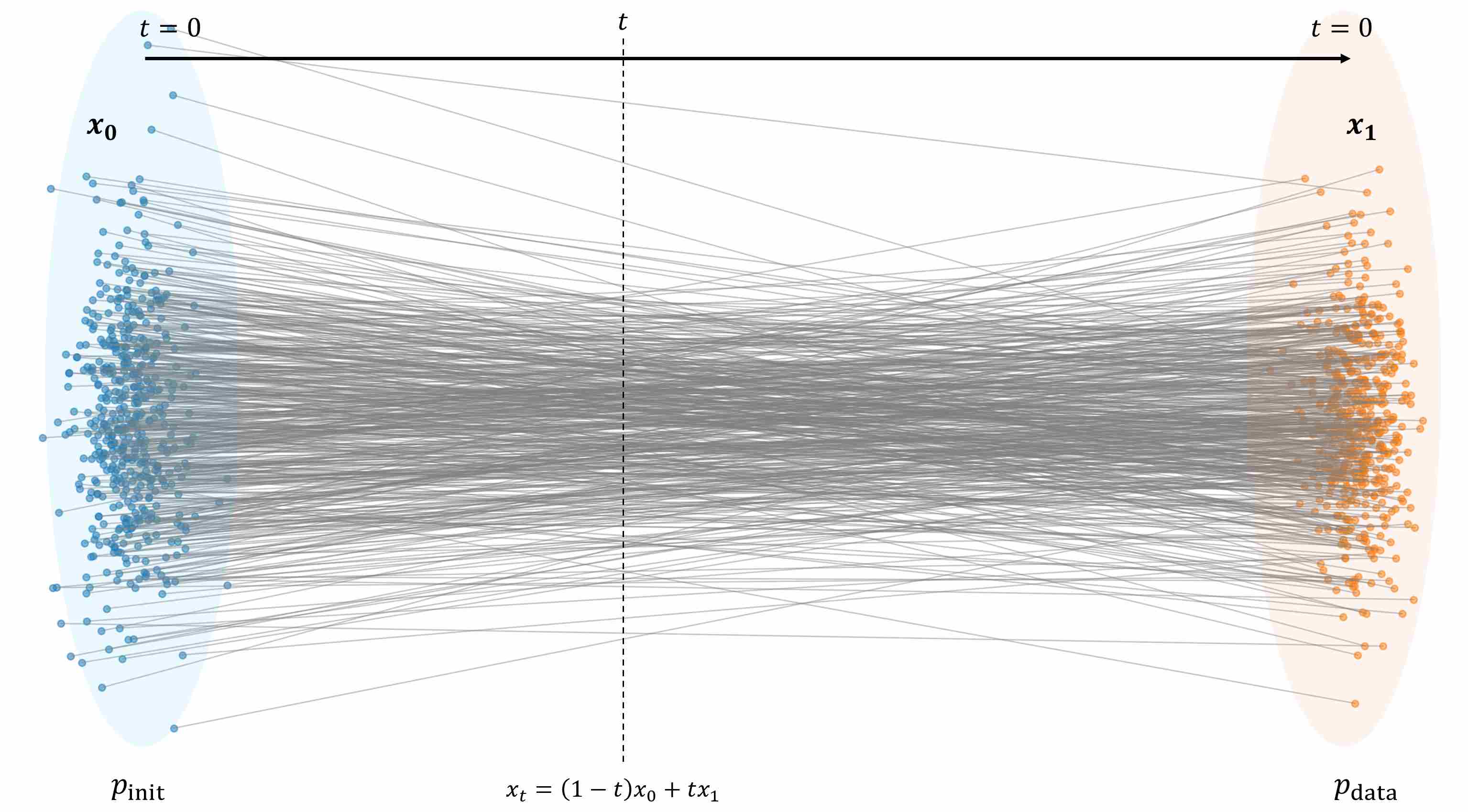
We had discussed Rectified Flow, a specifical case of FM, who defines the probability path as a straight line from the start point ($x_0 \sim p_{\text{init}}$) to the end point ($x_1 \sim p_{\text{data}}$) through linear interpolation. Therefore, in theory, RF can achieve one-step generation.

However, in practice, the trajectory of the ODE remains a curve. The core reason is thar the learned vector field is the average instantaneous velocity at each spatial point $x_t=x$ and time $t$:

Therefore, what the model learns is not the deterministic velocity of a specific straight-line path, but the conditional expectation of velocities across all possible paths at that point. The following figures shows the straight-line paths between different sample pairs.

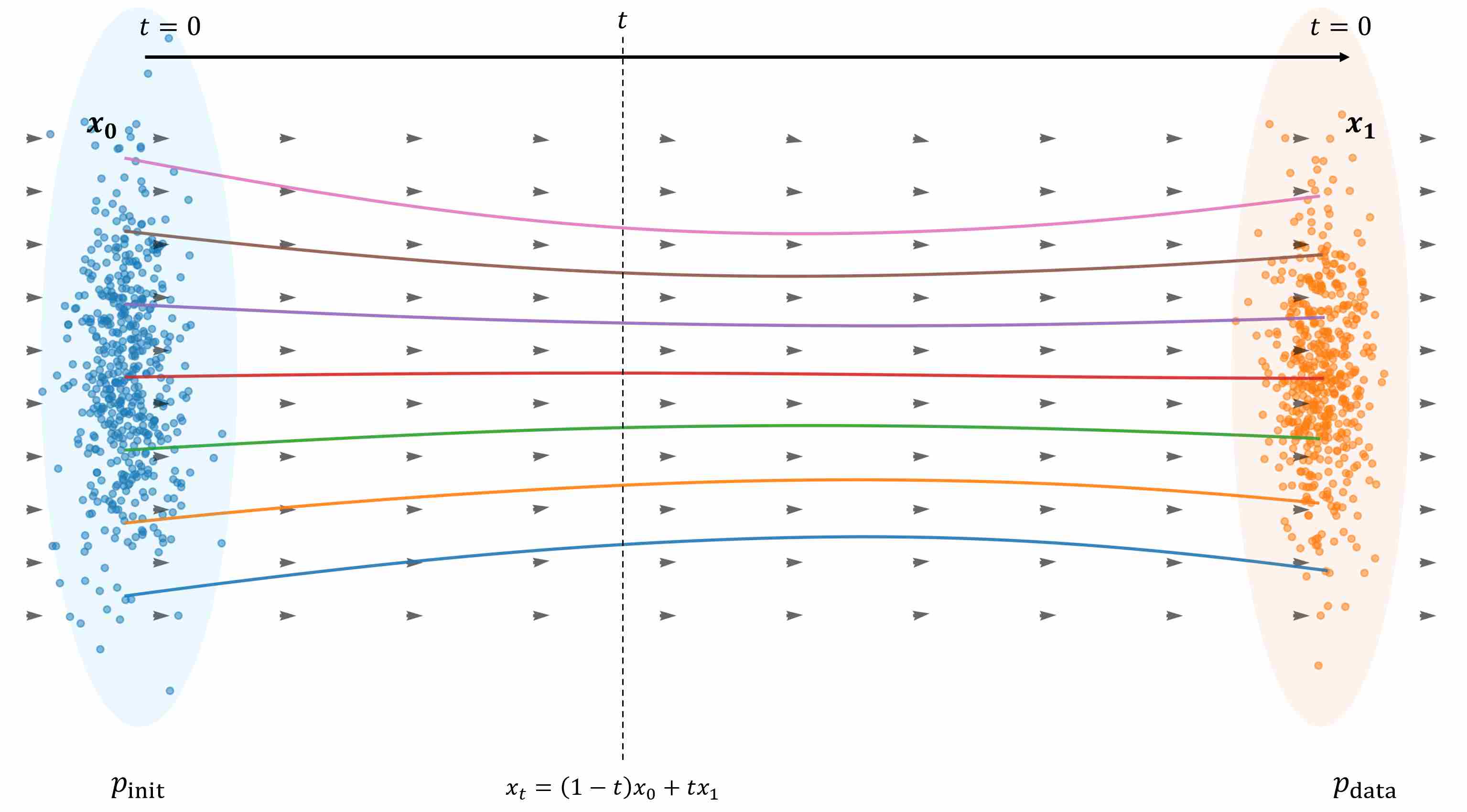
However, given this sample dataset, the obtained ODE trajectory is curved, as shown in the following figure.

2.1 Mathematical View

The Key Idea is that local averaging of velocities causes curvature: Many different pairs $(x_0, x_1)$ may pass near the same spatial location $x_t = x$, each with a different direction $x_1 - x_0$, when we take the average direction of all those local velocities, the resulting mean velocity vector depends on where $x$ is located.

Hence, the mean velocity field $v^\star(x, t)$ is spatially non-uniform — it bends, twists, and changes direction smoothly across space.

From a mathematical perspective, the mean velocity at location $x$ is:

where $p(x_0, x_1 \mid x_t = x)$ is conditional distribution of start ($x_0$) and end points ($x_1$) given the intermediate position ($x_t$), which is usually not a constant, because for different values of $x_t=x$, there are different pairs ((x_0, x_1)) passing through, which typically forms a very complex distribution. Thus, $v^\star(x, t)$ is not constant in space, and integrating it yields curved streamlines.

3. Reflow: iteratively training makes the path straighter

As we had mentioned above, the hidden curvature problem makes sampling procedure still relies on multi-step numerical integration. This discrepancy motivates ReFlow: an iterative method to straighten the learned trajectories and accelerate sampling.

ReFlow is an iterative self-distillation procedure applied on top of Rectified Flow. In practice, the first rectified flow $v_\theta^{(1)}$ learned from random couplings \((x_0, x_1) \sim p_0 \times p_1\) may not achieve perfect linearity. Thus, the authors propose ReFlow, an iterative self-distillation procedure:

1. Step 1: Use the current flow $v_\theta^{(k)}$ to generate new data pairs:

   \[x_1' = x_0' + \int_{0}^{1} v_\theta^{(k)}(t, x_t) dt, \quad (x_0' \sim p_0).\]

2. Step 2: Treat $(x_0’, x_1’)$ as new couplings and re-train:

   \[v_\theta^{(k+1)} = \arg\min_v \int_0^1 \mathbb{E}\big[|(x_1' - x_0') - v((1-t)x_0' + t x_1', t)|^2\big] dt. \tag{6}\]

Repeat the above steps, each iteration yields straighter trajectories and smaller transport cost.This process can be viewed as a geometry-level self-distillation: each generation acts as a teacher defining a more coherent flow geometry, while the student learns to approximate it using newly induced couplings.

3.1 Improving the Training: One Reflow is Sufficient

In practical settings, research ² indicated that the trajectory curvature of the optimal 2-rectified flow is actually close to zero. the linear interpolation paths of pairs generated by 1-Rectified Flow almost never intersect.

Suppose there are two points, $x_1\sim p_{\text{init}}$ and $x_2\sim p_{\text{init}}$, both sampled from the initial distribution, and the vector field obtained by 1-rectified flow is $v_{\theta}^1$. Then, following this vector field $v_{\theta}^1$, the sampling results for these two points are:

These two trajectories (\(x_1 \to z_1\) and \(x_2 \to z_2\)) almost never intersect. Since if two linear interpolation trajectories intersect, that implys that $z_2-z_1$ is parallel to $x_2-x_1$, which is almost impossible under high-dimension space.

This pivotal observation shifts the focus from adding more Reflow stages to perfecting the training of the 2-Rectified Flow itself. We can explain this in more detail,

• 1-Rectified Flow Training: at the beginning of Flow Matching training, we draw pairs

  \[(x_0, x_1) \sim \pi_0(x_0, x_1) = p_{\text{init}}(x_0) \times p_{\text{data}}(x_1),\]

  However, this coupling $\pi_0$ is random and unstructured — there is no consistent mapping between points in $p_0$ and $p_1$. Different sample pairs $(x_0, x_1)$ may cross in space, the optimal flow field

  \[v^\star(x,t) = \mathbb{E}[x_1 - x_0 \mid x_t = x]\]

  represents only the average direction across those mixed trajectories, hence the learned field $v_1$ is curved, because its direction varies spatially.

• 2-Rectified Flow Training: When we use $v_1$ to generate new samples:

  \[x_1^{(1)} = \Phi_{v_1}(x_0),\]

  where $\Phi$ is an ODE Solver, we create a new coupling \(\pi_1(x_0^{(1)}, x_1^{(1)})\) with two crucial properties:

  1. Deterministic mapping. Each $x_0^{(1)}$ maps to a unique endpoint $x_1^{(1)}$. Hence, $\pi_1$ is no longer a random or mixed coupling — it is now deterministic.

  2. Directional consistency. Along the ODE, the instantaneous velocity is fixed by the field $v_1(x_t, t)$, so all trajectories passing through the same point $x_t$ share the same direction. This eliminates local uncertainty:

     \[\mathrm{Var}(x_1^{(1)} - x_0^{(1)} \mid x_t) \approx 0.\]

  In other words, while $v_1$ may still appear curved in a global sense, the flow it induces is locally coherent — all particles follow the same vector field, removing the randomness in direction that caused curvature in the first place.

Unlike the 1-Rectified Flow training, the 2-Rectified Flow can be maximized the effectiveness by the following techniques.

• U-Shaped Timestep Distribution: The training difficulty for 2-Rectified Flow is not uniform across time t. The tasks at the endpoints—prediction at $t=0$ (from noise to image) and inversion at $t=1$ (from image back to noise)—are far more challenging than the interpolation task in the middle.

• Incorporating Real Data: Training 2-rectified flow does not require real data (i.e., it can be data-free), but we can use real data if it is available. mixing endpoints strategy: with probability $1-p$ take a real endpoint, with probability $p$ take a synthetic endpoint.

• Advanced Loss Function (LPIPS-Huber Loss): The original L2 loss is suboptimal for image generation as it often leads to blurry results and is sensitive to outliers. The new approach leverages the knowledge that the optimal flow is straight, allowing for more flexible loss functions.

4. InstaFlow: Text-Conditioned Rectified Flow with One-Step Distillation

In previous articles (Accelerating Diffusion Sampling), we introduced how to use distillation to accelerate the sampling of diffusion models. However, as we discussed in Sec. 1.1, diffusion models are based on the path strategy of SDEs, while PF-ODE being merely a by-product, which leads to suboptimal results in distillation. InstaFlow ³ extends this line of work by combining Rectified Flow with ReFlow and a final one-step distillation, transforming a large diffusion model (e.g., Stable Diffusion) into a high-quality, single-step flow generator.

4.1 Overview: From Stable Diffusion to One-Step Flow

InstaFlow can be viewed as a two-stage rectification and distillation pipeline:

1. Teacher Initialization: Start from a pretrained diffusion model (e.g., Stable Diffusion) and interpret its deterministic sampling process as a probability flow ODE:

   \[\frac{dx}{dt} = v_{SD}(x, t \mid T)\]

   where $T$ is the text condition. By integrating this ODE for 20–50 steps, the model generates pairs $(x_0, x_1)$ — noise to image mappings under given text conditions.

2. ReFlow Rectification: Apply Rectified Flow training on the collected dataset $(x_0, x_1, T)$, learning a smoother and more linear velocity field $v_{\theta}(x,t\mid T)$. This is the text-conditioned ReFlow stage, which regularizes the geometry of the generative flow under each prompt $T$.

3. Distillation to One-Step Flow: A student network $\tilde{v}(x_0\mid T)$ is trained to approximate the final displacement:

   \[x_1 \approx x_0 + \tilde{v}(x_0 \mid T)\]

   using a perceptual distance loss (LPIPS). This collapses the full ODE integration into a single Euler step, enabling instantaneous generation.

4.2 Text-Conditioned ReFlow

Unlike the original ReFlow which is unconditional, InstaFlow introduces text-conditioned Rectified Flow by conditioning $v(x,t)$ on textual embeddings $T$ through cross-attention. The training objective becomes:

where $x_1(T)$ is generated via the teacher Stable Diffusion model under the same text condition $T$. Each ReFlow iteration improves the local straightness of conditional trajectories without altering their marginal image distribution.

This step is essential because conditional generation introduces multiple sub-manifolds (different prompts induce different flow geometries). Text-conditioned ReFlow ensures each submanifold’s flow is straightened individually, preserving semantic alignment across conditions.

4.3 One-Step Distillation

After obtaining a 2-Rectified Flow teacher, InstaFlow performs a final distillation to a one-step generator. The student network learns a displacement field that directly maps noise to image:

where $D(\cdot, \cdot)$ denotes a perceptual similarity loss (e.g., LPIPS + Huber). The resulting model, InstaFlow, generates a 512×512 image in ~0.09 seconds with quality comparable to 20–50 step diffusion sampling.

4.4 Practical Insights and Limitations

In essence, InstaFlow extends ReFlow into the conditional domain and compresses the entire ODE integration into a single learned displacement. It demonstrates that rectifying and distilling a diffusion teacher can yield true one-step generation without sacrificing image quality.

• Text Coverage Issue: Since ReFlow training relies on data generated by Stable Diffusion, text conditions $T$ that are rarely sampled yield few training pairs $(x_0, x_1, T)$. As a result, InstaFlow inherits the coverage limitations of its teacher: performance degrades for rare or unseen prompts.

• Improvement Strategies: Expanding the prompt dataset, applying prompt resampling (e.g., CLIP-based diversity sampling), or self-distillation with prompt augmentation can mitigate this bias.

• Relation to Diffusion Distillation: The same limitation exists in all conditional distillation frameworks — missing conditions lead to poor generalization. InstaFlow emphasizes path rectification before distillation, which reduces geometric variance and improves knowledge transfer.

5. Shortcut Model: Few-Step Generation via Step-Conditioned

In Section 3, ReFlow progressively straightened the flow field to reduce curvature; in Section 4, InstaFlow distilled a rectified teacher into a one-step student to achieve direct generation. However, both still operate under a common assumption: the model is trained to predict an instantaneous velocity $v(x,t)$, but at inference time, when we attempt to generate samples using only a few or even a single step, we are effectively executing a finite-time jump. This mismatch between infinitesimal training and finite inference leads to systematic biases and degraded quality. The Shortcut model aims to close this gap by explicitly conditioning on the step size and learning the finite-interval displacement direction. In other words, it learns not how to move infinitesimally, but how to jump across a time interval directly.

5.1 Formulation and Motivation

the Shortcut model introduces an explicit conditioning variable — the step size $d\in(0,1]$ — and learns a field $s_\theta(x_t,t,d)$ that predicts the average direction over the time interval $[t, t+d]$:

When $d\to 0$, this recovers the original FM setting since the average velocity over an infinitesimal interval equals the instantaneous velocity:

But for larger $d > 0$, the network learns to compensate for curvature and multimodality by directly regressing the finite-time displacement. In this sense, the Shortcut field acts as a generalized velocity, simultaneously encompassing both small-step and large-step behaviors. The model learns not only local tangent information but also how to interpolate or “shortcut” across a segment of the trajectory.

The key insights is that: If the Shortcut field truly represents a physically consistent finite-step motion, then composing two half-steps of size $d$ should yield the same displacement as a single large step of size $2d$. To encode this additivity property, the following self-consistency identity is imposed:

where $x’_{t+d}=x_t + s(x_t,t,d)d$ is the predicted midpoint. This elegant identity can be interpreted as a discrete form of trajectory composition: the large-step direction equals the average of two consecutive small-step directions. Geometrically, this encourages the learned field to be smooth and consistent across scales of time, ensuring that predictions at different step sizes form a coherent hierarchy.

Unlike methods such as ReFlow or InstaFlow, which require generating teacher trajectories, this condition is imposed directly on the model’s own outputs, allowing end-to-end training without external supervision.

5.2 Training and Inference: Learning to Jump Consistently

The Shortcut training objective integrates two complementary components:

1. Small-step anchoring (FM base): For $d=0$, the model must recover the classical FM velocity:

   \[\mathcal L_{\text{FM}} = \mathbb E_{x0, x1, t} \| s_\theta(x_t,t,0) - (x_1 - x_0) \|^2.\]

2. Self-consistency across scales: For $d>0$, enforce the additive consistency constraint:

   \[\mathcal L_{\text{SC}} = \mathbb E_{d, t} \| s_\theta(x_t,t,2d) - s_{\text{tgt}} \|^2\]

   where

   \[s_{\text{tgt}} = \frac{1}{2}s_\theta(x_t,t,d) + \frac{1}{2}s_\theta(x'_{t+d},t+d,d).\]

In practice, we use stop-gradient or an EMA copy of the network to compute $s_{\text{tgt}}$ for stable bootstrapping.

The overall loss is:

At inference, the same model can be used for any number of steps $M$. Set $d=1/M$, and evolve:

This single model thus supports:

• One-step generation (M=1): Directly jumps from noise to data.
• Few-step generation (M∈{2,4,8}): Allows intermediate refinements.
• Multi-step generation (M≈64–128): Recovers high-fidelity sampling equivalent to standard FM.

Because $s_\theta(x,t,d)$ explicitly depends on $d$, the model automatically adjusts its prediction to different integration granularities. This yields robust behavior across sampling budgets without any retraining or distillation.

6. MeanFlow: Learning Mean Velocity Fields for One-Step Generation

Although Flow Matching (FM) and Rectified Flow (RF) have provided a unified ODE view of generative modeling, both still rely on instantaneous velocity fields $v(x_t, t)$ and therefore require numerical integration during sampling. When the integration step is coarse (e.g., 1–4 steps), numerical error accumulates rapidly because the marginal flow trajectories are not perfectly straight even if the conditional flow is linear. This limitation makes true one-step generation (1-NFE) difficult: the model is trained to predict a continuous-time velocity field but is asked to execute a large discrete jump during inference.

To overcome this structural mismatch, MeanFlow ⁴ proposes to replace the instantaneous velocity by its temporal average, thus directly learning a quantity that corresponds to a finite displacement rather than an infinitesimal one. By learning the mean velocity field

The relation between instantaneous velocity and mean velocity is shown as follows.

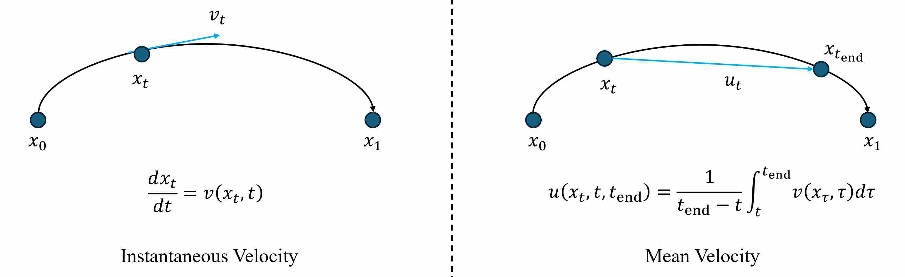
MeanFlow explicitly models the average motion between two time instants $t$ and $t_{\text{end}}$.

This design removes the need for numerical ODE integration: a single evaluation of (u) gives a displacement estimate capable of jumping directly from noise $(t{=}0)$ to data $(t_{\text{end}}{=}1)$.

6.1 MeanFlow Identity

Differentiating the definition of $u$ with respect to $t$ gives

Applying the product rule to the left side, leading to the MeanFlow Identity

This equation forms the theoretical foundation of MeanFlow: it expresses the instantaneous velocity in terms of the mean velocity and its total derivative. Conversely, the identity uniquely determines $u$ given $v$ and vice versa.

The total derivative $\tfrac{d}{dt}u(x_t, t, t_{\text{end}})$ contains both explicit and implicit time dependence, using chain rule gives

This is a Jacobian-vector product (JVP) that can be efficiently computed with modern autodiff frameworks (PyTorch, JAX) without incurring second-order gradient cost, as gradients are detached from the target branch.

6.2 Training Objective

Let $u_\theta(x_t, t, t_{\text{end}})$ denotes the neural network predicting the mean velocity. Substituting Eq. \ref{eq:meanflow2} into Eq. \ref{eq:meanflow1} yields a regression target:

When $t_{\text{end}}{=}t$, the second term vanishes and the loss degenerates to Flow Matching, ensuring compatibility. The training loss is a simple mean-squared error:

Sampling is simple, only one forward pass through $u_\theta$ suffices to map pure noise ($x_0=\epsilon$) to data.

6.3 MeanFlow vs Shortcut: Continuous Theory vs Discrete Realization

MeanFlow and Shortcut address the same pain point—high-quality few/one-step generation—by learning interval information instead of relying solely on instantaneous velocities as in classic Flow Matching (FM) or Rectified Flow (RF). Conceptually:

• MeanFlow is a continuous-time formulation: it defines and learns an average velocity field over a time interval, derived from first principles of the probability flow ODE.

• Shortcut is a discrete-time realization: it learns a finite-step displacement direction and enforces self-consistency across steps—behaving like a learned, problem-adapted numerical integrator for the same underlying ODE.

With $t_{\text{end}}=t+d$:

Hence, Step size $d$ in Shortcut is equal to interval length $(t_{\text{end}}-t)$ in MeanFlow. One-step sampling

6.3.1 Neural Integrator View: Shortcut as a Family of RK-like Schemes

We can also understand the relationship between meanflow and shortcut from the perspective of numerical integration. Specifically, if we regard meanflow as a continuous ODE, then shortcut is a type of discrete solution method for this ODE.

Interpreting $s_\theta$ as a learned local average velocity, Shortcut’s target can be generalized to emulate classic ODE integrators:

• Trapezoidal / Midpoint (2nd-order) — current common form

  \[s_{\text{tgt}}=\frac{1}{2}\,s_\theta(x_t,t,d)+\frac{1}{2}\,s_\theta(x_{t+d},t+d,d)\]

• Heun / Improved Euler (2nd-order)

  \[s_{\text{tgt}}=\frac{2}{3}\,s_\theta(x_t,t,\tfrac{2}{3}d)+\frac{1}{3}\,s_\theta(x_{t+\tfrac{2}{3}d},t+\tfrac{2}{3}d,\tfrac{1}{3}d)\]

• General RK-style template

  \[s_{\text{tgt}}=\sum_{i=1}^k w_i\,s_\theta\!\big(x_{t+\alpha_i d},\,t+\alpha_i d,\,\beta_i d\big), \quad \sum_i w_i=1,\]

  where the nodes/weights $(\alpha_i,\beta_i,w_i)$ define accuracy/stability trade-offs.

In summary, MeanFlow provides the continuous target—the interval average (u). Shortcut instantiates a discrete quadrature of that average with learnable evaluations of $s_\theta$ at selected nodes.

8. References