
From Diffusion to Flow: A New Genrative Paradigm
📅 Published:
📘 TABLE OF CONTENTS
- 1. Introduction: Seeking the Third Road of Generation
- 2. Mathematical Preliminaries and Core Concepts
- 3. Foundations of the Flow Matching Paradigm
- 4. Conditional Flow Matching: Making the Objective Tractable
- 5. Flow Matching and Score Matching: Two Sides of the Same Coin
- 6. Rectified Flow: A Linear Implementation of Flow Matching
- 7. Stochastic Interpolants: A Unified Framework for Flows and Diffusions
- 8. References
In the previous article (Accelerating Diffusion Sampling: From Multi-Step to Single-step Generation), we traced the evolution of fast diffusion sampling techniques—from numerical acceleration by high-order ODE solvers, to model-level acceleration via distillation, and finally to training-level acceleration embodied by Flow Matching.
In this article, we dives deeper into why Flow Matching achieves that acceleration by design. In doing so, we establishes and unfolds the foundations of Flow Matching: how it bridges diffusion and continuous normalizing flows, how it reframes generation as learning deterministic currents of transformation between distributions. These theoretical analyses ultimately build flow matching as a novel “path-first” generation paradigm.
1. Introduction: Seeking the Third Road of Generation
Before we arrive at Flow Matching itself, it is essential to understand the two dominant paradigms that shaped the landscape of modern generative modeling: diffusion models and normalizing flows. Each offers a distinct philosophy — diffusion relies on stochastic forward processes and iterative denoising, while flows construct invertible mappings grounded in probability theory. Both reveal valuable insights but also expose fundamental limitations. By examining their strengths and bottlenecks, we prepare the ground for a third road - Flow Matching.
1.1 The Rise and Bottlenecks of Diffusion Models
Diffusion models have defined the state of the art in generative modeling. By gradually adding noise through a fixed forward process and then learning to reverse it, they can approximate extremely complex data distributions with remarkable fidelity. We have discussed many training and sampling techniques for diffusion models in the previous posts.
However, their reliance on iterative denoising is costly. Sampling often requires hundreds of steps, each invoking a deep network, which makes inference slow and error-prone. The method is powerful but simulation-heavy, as both training (via noisy forward diffusion) and inference (via numerical solvers) depend on repeatedly simulating stochastic dynamics.
1.2 The Elegance and Constraints of Continuous Normalizing Flows
At the heart of Normalizing Flows (NFs) 1 2 3 lies a simple but powerful principle: the change-of-variables formula. It connects the density of a data point (denoted as $z$) in one space to the density of its transformed representation in another (denoted as $x$).
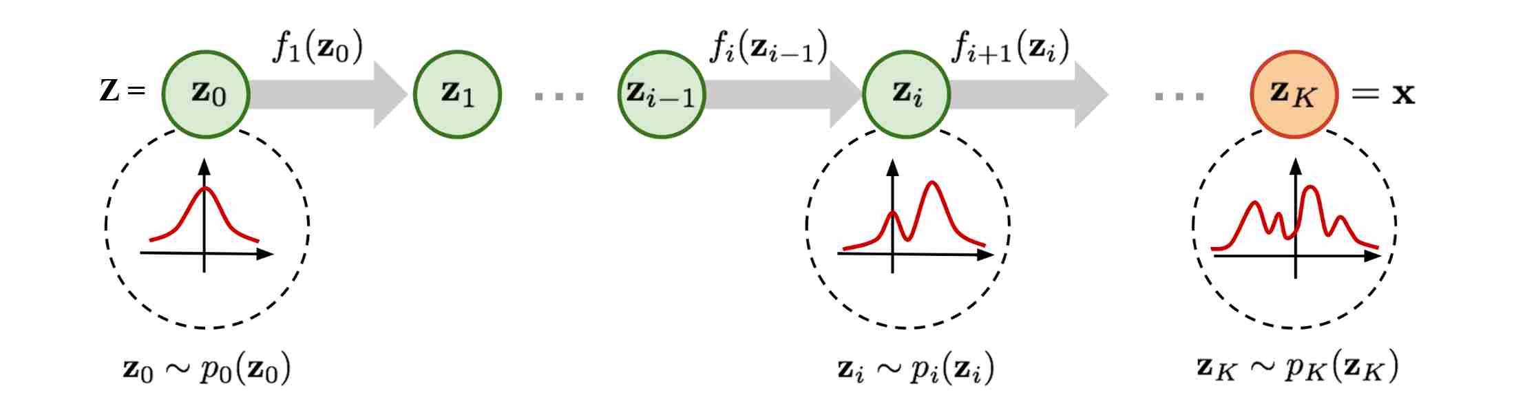
Suppose we have a random variable $z \sim p(z)$, where $p_z$ is a simple Gaussian distribution, we then construct a chain of $K$ invertible mappings ($\,f_i\,:\,\mathbb R^d \to \mathbb R^d\,$):
\[z_0 \sim p_z(z_0), \quad z_1 = f_1(z_0), \quad \dots, \quad x = z_K = f_K \circ \cdots \circ f_1(z_0).\]By repeatedly applying the change-of-variables formula, we get the final variable $x \sim p(x)$, the density of $x$ is given by
\[\log p(x) = \log p(z_0) - \sum_{k=1}^K \log \left|\det J_{f_i}\right|.\]Where $J_{f_i}$ is Jacobian Matrix. Thus, the entire model is exact likelihoods mathematically, as long as each transformation is invertible and its Jacobian determinant is tractable. However, the computation the Jacobian determinant of $f_i$ is very expensive in high dimensions.
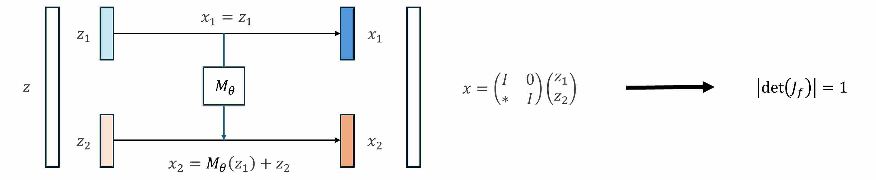
To make Jacobian computation feasible, invertible mappings should be designed for special architecture to guarantee a tractable Jacobian determinant. For example, Nice 1 using additive coupling layer to make Jacobian determinant is equal to 1.
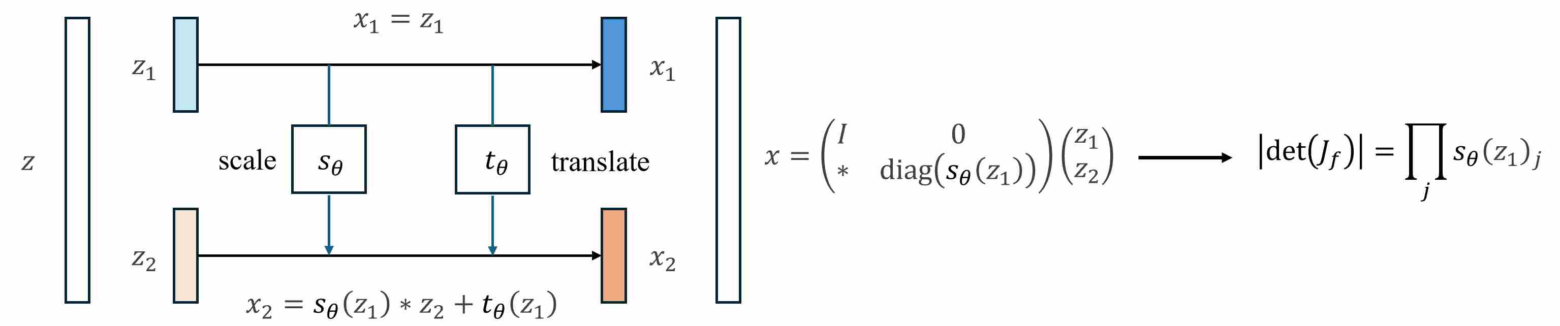
Real NVP 2 extends NICE’s additive coupling to an affine coupling layer, which guarantees that the Jacobian determinant is just the product of elementwise scales (a diagonal matrix). This makes log-likelihood tractable while keeping the model invertible and expressive.
The move from discrete transformations to continuous-time transformations gave rise to Continuous Normalizing Flows (CNFs) 4 5. Instead of stacking finitely many mappings, we let the transformation evolve under an ODE:
\[\frac{dx_t}{dt} = v_\theta(x_t, t), \quad x_0 \sim p_z, \quad x_1 \sim p_x.\]The corresponding density evolution is given by the instantaneous change-of-variables formula 4:
\[\frac{d}{dt} \log p(x_t) = - \text{Tr}\!\left(\frac{\partial v_\theta(x_t,t)}{\partial x_t}\right).\]In theory, CNFs remove the architectural rigidity of discrete NFs, allowing any sufficiently expressive neural network to parameterize the vector field $v_\theta$. They provide a mathematically elegant and continuous-time perspective on generative modeling, bridging flows and differential equations. CNF makes the entire model is exact likelihoods mathematically.
\[\log p(x_1)\,=\,\log p(x_0) - \int_{0}^{1} \text{Tr}\!\left(\frac{\partial v_\theta(x_t,t)}{\partial x_t}\right) dt\label{eq:cnf}\]Eq. \ref{eq:cnf} shows that the model’s log-likelihood depends on the entire trajectory of the ODE. To evaluate this term—or its gradient during training—we must numerically integrate both the state equation and the divergence over continuous time, since no closed-form expression of $x_t$ or the integral exists. Therefore, maximum-likelihood training of CNFs necessarily requires calling an ODE solver to trace how each sample evolves through the continuous flow and accumulate the corresponding log-density change.
Together, these factors make CNF training orders of magnitude slower than discrete flows or flow-matching methods, which avoid integrating through the ODE during training.
1.3 The Breaking Point: Toward Direct Paths Between Distributions
Between diffusion’s slow stochastic wanderings and CNF’s constrained elegance lies a natural question: must generative modeling always depend on heavy simulation or exact density tracking?
Imagine instead that we could directly learn the transformation path between two distributions — for example, between noise and data. Rather than simulating a process step by step, or computing exact likelihoods, we could regress a vector field that prescribes how samples should flow from one distribution to another. This reframes generative modeling as the study of currents of transformation, where the emphasis shifts from simulation to direct learning.
This insight marks the turning point for Flow Matching. It signals the possibility of a third road: a paradigm that is at once intuitive, efficient, and theoretically unifying.
2. Mathematical Preliminaries and Core Concepts
Flow-based models are grounded in the interplay between geometry and probability—how distributions evolve along vector fields through time. Before delving into the specifics of flow matching, we need to formalize these fundamental geometric components: the notion of a vector field, the trajectory traced by particles under its influence, and the resulting flow of probability mass across time.
Understanding these objects is crucial, because flow matching does not define a stochastic diffusion process; rather, it constructs deterministic trajectories that guarantee probability conservation via the continuity equation. The following subsection introduces these mathematical building blocks.
2.1 Vector Fields, Trajectories, and the Dynamics of Flow
Vector Field: vector field is a function that assigns to each spatial point $x_t \in \mathbb R^d$ and time $t \in [0, 1]$ an instantaneous velocity $v_{\theta}(t, x_t)$:
\[v_{\theta}:\ \mathbb R^d \times [0,1] \to \mathbb R^d\label{eq:1}\]ODE: ODE (Ordinary Differential Equation) is the dynamical law you impose using that vector field:
\[\frac{dx_t}{dt}=v_{\theta}(t, x_t)\label{eq:2}\]Solving this ODE from $t=0$ to $t=1$ is equivalent to sampling, whose goal is to transport an initial point $x_0$ to a target $x_1$ through space according to the learned velocities.
Trajectory: A trajectory $(x_0, \dots, x_{t}, \dots,x_1)$, is simply the solution of the above ODE for a given start point $x_0$. It’s the continuous path that the “particle” traces out under the influence of the vector field:
\[x(t)=x(0) + \int_0^tv_{\theta}(s, x(s))ds\label{eq:3}\]Or using the Euler method to solve in a discrete time step ($\,h=t_n-t_{n-1}\,$):
\[x_{t_n}\,=\,x_{t_{n-1}} \,+\, h \times v_{\theta}(t_{n-1}, x_{t_{n-1}})\label{eq:4}\]Flow: a flow is essentially a collection of trajectories that follows the ODE, that means by solving the above ODE we gather a lot of solutions for different initial points
2.2 Defining Probability Paths Between Distributions
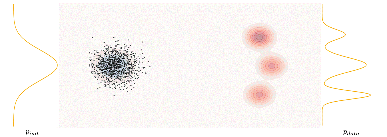
The first step of FM is to define a probability path, who specifies a gradual interpolation from initial distribution $p_{init}$ to target distribution $p_{\text data}$.
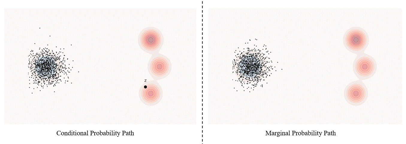
Conditional probability path: given an end point $z \sim p_{\text data}$, a conditional probability path is the distribution of an intermediate sample conditioned on $z$, denoted as $p_t(x_t \mid z)$ such that
\[p_0(\cdot \mid z)=p_{init},\ \ \ p_0(\cdot \mid z)=\delta_z \ \ \ \ {\rm for\ all}\ z \in \mathbb R^d\label{eq:5}\]Marginal probability path: marginal probability path defined as the distribution that we obtain by first sampling a data point $z ∼ p_{\text data}$ from the data distribution and then sampling from $p_t(x_t |z)$, we can formalize it as:
\[p_t(x_t)=\int p_t(x_t|z) p_{\text data}(z)dz\label{eq:6}\]$p_t(x_t)$ satisfy $p_0(\cdot)=p_{init}$ and $p_1(\cdot)=p_{data}$. The difference between the marginal probability path and the conditional probability path can be illustrated as follows.
Please be noticed that, in diffusion models, it is more common to use $x_0$ to represent the clear original image and $x_1$ to represent noise; whereas in flow matching, the opposite is true, with $x_1$ more commonly used to represent the clear original image and $x_0$ to represent noise.
In the following, I will use $ p_0 $ or $ p_{\text{init}} $ to denote the initial distribution; $ p_1 $ or $ p_{\text{data}} $ to denote the true data distribution; $ p_t $ to denote the distribution at an intermediate time $0 < t < 1$.
3. Foundations of the Flow Matching Paradigm
Diffusion model relies on the forward process, from which the reverse denoising SDE and PF-ODE are derived, which we refer to as the “process-first” generative paradigm. The core of Flow Matching (FM) 6, however, is to construct a probability path that connects the initial distribution $p_0$ to the target distribution $p_1$, which we refer to as the “path-first” generative paradigm.
3.1 Marginal Probability Paths and Their Induced Vector Fields
Flow Matching begins by defining a more general marginal probability path, $x_t \sim p_t(x_t)$, that connects any pair of points $x_0 \sim p_0$ (noise) and $x_1 \sim p_1$ (data).
\[x_t = \alpha(t)x_0+\beta(t)x_1,\quad t\in[0,1]\label{eq:15}\]This path is a time-dependent probability distribution that satisfies the boundary conditions:
- at $t=0$, it concentrates on the starting point: $x_0 \sim p_0$.
- at $t=1$, it concentrates on the endpoint: $x_1 \sim p_1$.
Associated with this probability path is a marginal vector field, $v_t(x_t)$, which represents the instantaneous velocity required for a particle at position $x_t$ at time $t$ to stay on the trajectory defined by the path.
\[v_t(x_t) = \frac{dx_t}{dt} = \frac{d\alpha(t)}{dt}x_0 + \frac{d\beta(t)}{dt}x_1\]This temporal path of marginals can be realized by ODE dynamic: defining the probability-flow ODE via this velocity field.
\[\frac{dx_t}{dt} = v_t(x_t)\label{eq:17}\]under the continuity equation, we guarantees that, at each time $t$ , the marginal distribution of $x_t$ obtained by solving the ODE, is exactly follows the marginal distribution $p_t$ described in \ref{eq:15}.
3.2 Ensuring Consistency through the Continuity Equation
Now let’s prove why the ODE defined by the velocity field produces exactly the prescribed marginal densities $p_t$.
Step 1: The marginal path defined in Eq. \ref{eq:15} satisfies the continuity equation
Prove: Take any smooth, compactly supported test function $\varphi:\mathbb{R}^d\to\mathbb{R}$. By the chain rule and our assumptions,
\[\begin{align} \frac{d}{dt}\,\mathbb{E}\big[\varphi(x_t)\big] = \mathbb{E}\big[\nabla_x\varphi(x_t)\cdot \partial_t x_t\big]. \end{align}\]Disintegrate (i.e., condition on $x_t$):
\[\begin{align} \mathbb{E}\big[\nabla_x\varphi(x_t)\cdot \partial_t x_t\big] & = \int \nabla_x\varphi(x_t)\cdot \underbrace{\mathbb{E}\big[\partial_t x_t\mid x_t=x\big]}_{v_t(x)}\, p_t(x)\,dx \\[10pt] & = \int \nabla_x\varphi(x)\cdot \big(p_t(x)v_t(x)\big)\,dx \\[10pt] & = -\int \varphi(x)\,\nabla_x\!\cdot\!\big(p_t(x)u_t(x)\big)\,dx\label{eq:47} \end{align}\]On the other hand,
\[\frac{d}{dt}\,\mathbb{E}\big[\varphi(x_t)\big] = \frac{d}{dt}\int \varphi(x)\,p_t(x)\,dx = \int \varphi(x)\,\partial_t p_t(x)\,dx.\label{eq:48}\]Compare Eq. \ref{eq:48} and Eq. \ref{eq:47}, it can be derived
\[\int \varphi(x)\,\partial_t p_t(x)\,dx = -\int \varphi(x)\,\nabla_x\!\cdot\!\big(p_t(x)v_t(x)\big)\,dx.\]Because this holds for all test functions $\varphi$, we obtain the continuity equation in weak (and hence classical) form:
\[\boxed{ \;\partial_t p_t(x) + \nabla_x\!\cdot\!\big(p_t(x)\,v_t(x)\big) = 0.\; }\]This is simply conservation of probability mass under the velocity field $v_t$.
Step 2: The ODE’s law (Eq. \ref{eq:17}) satisfies the same continuity equation
Prove: Consider the probability-flow ODE
\[\frac{dx_t}{dt} \;=\; v_t(x_t), \qquad x_0 \sim p_0.\]Under standard conditions (e.g., $v_t(\cdot)$ globally Lipschitz in $x$, measurable in $t$), the ODE has a unique solution, and $x_t$ is a measurable function of $x_0$. Let $\mu_t$ denote the law (density) of $x_t$. Repeat the same test-function computation:
\[\begin{align} \frac{d}{dt}\,\mathbb{E}\big[\varphi(x_t)\big] & = \mathbb{E}\big[\nabla_x\varphi(x_t)\cdot \frac{dx_t}{dt}\big] = \mathbb{E}\big[\nabla_x\varphi(x_t)\cdot v_t(x_t)\big] \\[10pt] & = \int \nabla_x\varphi(x)\cdot\big(\mu_t(x)v_t(x)\big)\,dx \\[10pt] & = -\int \varphi(x)\,{\nabla_x} \cdot \big(\mu_t v_t\big)\,dx. \end{align}\]Similar to Eq. \ref{eq:48}, we also have
\[\frac{d}{dt}\mathbb{E}[\varphi(x)]=\int \varphi(x)\,\partial_t \mu_t(x)\,dx\]Hence
\[\int \varphi\,\partial_t \mu_t dx = -\int \varphi\,\nabla_x\!\cdot(\mu_t v_t) dx \quad\Longrightarrow\quad \boxed{ \;\partial_t \mu_t + \nabla\!\cdot(\mu_t v_t)=0.\; }\]So $\mu_t$ satisfies the same continuity equation with the same velocity field $v_t$ and the same initial density $\mu_0=p_0$. Therefore,
\[\boxed{ \quad \mu_t \equiv p_t \quad \text{for all } t\in[0,1]. \quad }\]
In words: the ODE driven by $v_t$ produces exactly the prescribed path of marginals.
3.3 Core Objective: Learning the Target Vector Field via Regression
With a general path $p_t$ and its target vector field $v_t(x_t)$ defined, the learning problem becomes remarkably direct. The goal is to train a neural network $v_\theta(x_t, t)$ to match the target vector field $v_t$ at any time step $t$. This is formulated as the Flow Matching objective:
\[\mathcal{L}_{\text{FM}}(\theta) = \mathbb{E}_{t \sim \mathcal{U}[0,1],\, x_t \sim p_t} \big[\, \| v_\theta(x_t, t) - v_t(x_t) \|^2 \,\big]\label{eq:18}\]3.4 Translating Perspectives: Bridging CNF, PF-ODE, and FM
Flow Matching does not exist in a vacuum. It provides a new lens through which we can understand and unify existing paradigms.
Connection to Continuous Normalizing Flows (CNFs): Both FM and CNFs learn a vector field $v_\theta$ to define a continuous-time generative model. However, CNFs are trained via maximum likelihood, which requires computing the computationally expensive Jacobian trace ($\text{Tr}(\nabla_x v_\theta)$). Flow Matching cleverly sidesteps this. The FM objective is a regression loss that is mathematically proven to guide the marginal probability path $p_t(x)$ to match the target data distribution, effectively achieving the same goal as CNFs but without the need for trace computations. It trades the exact likelihood objective for a more direct and scalable vector field regression.
Connection to Probability Flow ODEs (PF-ODEs): Diffusion models also have a corresponding deterministic ODE for sampling, known as the Probability Flow ODE. This ODE’s vector field is derived from the score of the noisy data distribution. To train a model to predict this score, one must simulate the forward stochastic noising process. Flow Matching provides a more direct route. It bypasses the need for a stochastic process and score estimation entirely by directly defining the desired path and regressing its vector field. While both frameworks ultimately yield a generative ODE, FM constructs it from a “path-centric” perspective, whereas diffusion arrives at it from a “process-centric” one.
By establishing this simple, scalable regression objective, Flow Matching created a powerful new paradigm for generative modeling—one that retains the continuous-time elegance of CNFs while offering the practical efficiency and performance of diffusion models.
4. Conditional Flow Matching: Making the Objective Tractable
While Flow Matching provides a general regression framework, optimizing the target function shown in Equation \ref{eq:18} is very difficult, as directly estimating true target $v_t(x_t)$ is expensive: it requires integrating over all possible $z \sim p_{1}$ that generated by $x_t$.
\[v_t(x_t)=\int v_t(x_t|z)p(z|x_t)dz=\int v_t(x_t|z)\frac{p_t(x_t|z)p_{\text data}(z)}{p(x_t)}dz\label{eq:19}\]Conditional Flow Matching (CFM) solves this problem by introducing a conditioning variable $z$ that makes the velocity target explicit and unbiased, while avoiding marginalization over all possible samples.
CFM begins by defining Conditional probability path ($2.2), $p_t(x_t \mid z)$, Here, $z$ is deterministic data sampled from $p_{\text data}$, rather than arbitrary data. Similarly, associated with this probability path is a Conditional vector field, $v_t(x_t \mid z)$, the relationship between Conditional vector field and marginal vector field is as shown in \ref{eq:19}.
Now, with the conditional vector field as the true target, we construct the objective function for CFM.
\[\mathcal L_{\text{CFM}}(\theta)= \mathbb{E}_{t \sim \mathcal{U}[0,1],\, z\sim p_{\text data},\, x_t \sim p_t(\cdot \mid z)} \big|\big| v_{\theta}(t, x_t) - v_t(x_t|z) \big|\big|^2\label{eq:22}\]Conditional velocity field is tractable, which makes it feasible to minimize $\mathcal L_{\text{CFM}}(\theta)$ mathematically. Now let’s analyze why optimizing $\mathcal L_{FM}$ and optimizing $\mathcal L_{\text{CFM}}$ yield the same optimal vector field.
\[\begin{align} & \mathcal L_{FM}(\theta)=\mathbb E_{\scriptscriptstyle t\sim U(0,1), x_t\sim p_t(x_t)}\| v_{\theta}(t, x_t) - v_t(x_t) \|^2\label{eq:23} \\[10pt] \Longrightarrow \quad & \mathcal L_{FM}(\theta)=\mathbb E_{\scriptscriptstyle t \sim U(0,1), x_t\sim p_t(x_t)}\big(\| v_{\theta}(t, x_t) \|^2 -2\| v_{\theta}(t, x_t) \| \| v_t(x_t) \| + \| v_t(x_t) \|^2 \big) \quad \label{eq:24} \end{align}\]Consider the second term:
\[\begin{align} & \mathbb E_{t\sim U(0,1), x_t\sim p_t(x_t)}\big(\| v_{\theta}(t, x_t) \| \times \| v_t(x_t) \| \big)\label{eq:25} \\[10pt] \Longrightarrow \quad & \int_t\int_{x_t} p_t(x_t) \times \| v_{\theta}(t, x_t) \| \times \| v_t(x_t) \|dx_tdt\label{eq:26} \\[10pt] \Longrightarrow \quad & \int_t\int_{x_t} p_t(x_t) \times \| v_{\theta}(t, x_t) \| \times \big( \int_z \underbrace{\| v_t(x_t|z) \| \times \frac{p_t(x_t \mid z)p_{\text data}(z)}{p(x_t)}}_{\text{Eq. 33}} dz \big) dx_tdt\label{eq:27} \\[10pt] \Longrightarrow \quad & \int_t\int_{x_t}\int_z p_t(x_t) \times \frac{p_t(x_t \mid z)p_{\text data}(z)}{p(x_t)} \times \| v_{\theta}(t, x_t) \| \times \| v_t(x_t \mid z) \|dzdx_tdt\label{eq:28} \\[10pt] \Longrightarrow \quad & \int_t\int_{x_t}\int_z p_t(x_t \mid z) \times p_{\text data}(z) \times \| v_{\theta}(t, x_t) \| \times \| v_t(x_t \mid z) \|dzdx_tdt\label{eq:29} \\[10pt] \Longrightarrow \quad & \mathbb E_{\scriptscriptstyle t\sim U(0,1), z\sim p_{\text data}(z), x_t\sim p_t(x_t|z)}\big(\| v_{\theta}(t, x_t) \| \times \| v_t(x_t \mid z) \| \big)\label{eq:30} \end{align}\]Now, Let’s substitute the second item with the result above:
\[\begin{align} & \mathcal L_{\text{FM}}(\theta)=\mathbb E_{\scriptscriptstyle t ,\, x_t }\| v_{\theta}(t, x_t) - v_t(x_t) \|^2 \\[10pt] \Longrightarrow \quad & \mathcal L_{\text{FM}}(\theta)=\mathbb E_{\scriptscriptstyle t ,\, x_t}\big(\| v_{\theta}(t, x_t) \|^2 -2\| v_{\theta}(t, x_t) \| \| v_t(x_t) \| + \| v_t(x_t) \|^2 \big) \\[10pt] \Longrightarrow \quad & \mathcal L_{\text{FM}}(\theta)=\mathbb E_{\scriptscriptstyle t,\,z,\,x_t}\big(\| v_{\theta}(t, x_t) \|^2 -2\| v_{\theta}(t, x_t) \| \| v_t(x_t \mid z) \| + \| v_t(x_t) \|^2 \big) \quad \\[10pt] \Longrightarrow \quad & \mathcal L_{\text{FM}}(\theta)=\mathbb E_{\scriptscriptstyle t,\,z,\,x_t}\| v_{\theta}(t, x_t) - v_t(x_t|z) \|^2 +C_1+C_2 \\[10pt] \Longrightarrow \quad & \mathcal L_{\text{FM}}(\theta) = \mathcal L_{\text{CFM}}(\theta)+C \end{align}\]where
\[\begin{align} & C_1 = \mathbb E_{\scriptscriptstyle t\sim U(0,1), z\sim p_{\text data}(z), x_t\sim p_t(x_t|z)}\big[ \| v_t(x_t)\|^2\big] \\[10pt] & C_2 = \mathbb E_{\scriptscriptstyle t\sim U(0,1), z\sim p_{\text data}(z), x_t\sim p_t(x_t|z)}\big[ -\| v_t(x_t \mid z)\|^2\big]\label{eq:cfm} \end{align}\]Since $C_1$ and $C_2$ are independent with the parameters $\theta$, their derivatives will be zero. In the context of gradient updates, these two terms can be treated as constants. Eq. \ref{eq:cfm} shows that minimizing $\mathcal L_{\text{FM}}$ is equal to minimizing $\mathcal L_{\text{CFM}}$ with represpect to $\theta$.
5. Flow Matching and Score Matching: Two Sides of the Same Coin
In diffusion models, we use SDEs to unify two different implementations: discrete Markov denoiser and Langevin dynamics, where the score is the core of SDE-based diffusion models.
Specifically, given diffusion forward process:
\[x_t = s(t)z + \sigma(t)\epsilon, \quad z \sim p_{\text{data}}\, \text{and}\, \epsilon \sim \mathcal N(0, I)\]where $x_t \sim p_t(x)$, referring to the definition of the marginal vector field, the marginal score is the gradient of the log-density with respect to $x$
\[\nabla_x \log p_t(x)\in\mathbb{R}^d.\]Similarly, suppose $x_t$ is conditionally distributed given a latent $z$ with conditional density $p_t(x\mid z)$. The conditional score is
\[\nabla_x \log p_t(x\mid z).\]The relationship between the marginal score and the conditional score is analogous to that between the marginal vector field and the conditional vector field (Eq. \ref{eq:19})
\[\begin{align} \nabla_x \log p_t(x) & =\frac{\nabla_x p_t(x)}{p_t(x)} = \int \frac{\nabla_x p_t(x\mid z)\,p(z)}{p_t(x)}\,dz \\[10pt] & = \int \nabla_x \log p_t(x\mid z) \frac{p_t(x\mid z)\,p(z)}{p_t(x)}\,dz \end{align}\]Let us first consider the relationship between the conditional vector field and the conditional score.
\[\begin{align} v_t(x\mid z) & = \frac{dx}{dt} = \dot{s}(t)z+\dot{\sigma}(t)\frac{x-s(t)z}{\sigma(t)} \\[10pt] & = \frac{\dot{s}(t)}{s(t)}\,x + \frac{\dot{s}(t)}{s(t)}\,\sigma(t)^2\,\left(- \frac{x-s(t)z}{\sigma^2(t)} \right) - \dot{\sigma}(t)\sigma(t)\,\left(- \frac{x-s(t)z}{\sigma^2(t)} \right) \\[10pt] & = \frac{\dot{s}(t)}{s(t)}\,x + \Big(\frac{\dot{s}(t)}{s(t)}\,\sigma^2(t) - \dot{\sigma}(t)\,\sigma(t)\Big) \nabla_x \log p_t(x \mid z). \end{align}\]where we use
\[\dot{s}(t) = \frac{ds(t)}{dt}\qquad \text{and}\qquad \dot{\sigma}(t) = \frac{d\sigma(t)}{dt}\]for the convenience of writing. This equality also holds for the marginal distribution.
\[v_t(x) = \frac{\dot{s}(t)}{s(t)}\,x + \Big(\frac{\dot{s}(t)}{s(t)}\,\sigma^2(t) - \dot{\sigma}(t)\,\sigma(t)\Big) \nabla_x \log p_t(x).\label{eq:sm_fm}\]Eq. \ref{eq:sm_fm} shows that the vector field $v_t(x)$ is a linear transformation of the score $\nabla_x \log p_t(x)$ and the position $x$. This relation implies that, under Gaussian paths, the velocity field $v_t(x)$ and score field $\nabla_x \log p_t(x)$ encode the same geometric information about the evolving density $p_t(x)$.
Recalling our previous article, we mentioned that given a forward SDE, we can derive the corresponding reverse SDE, and from the reverse SDE, we can derive the equivalent PF-ODE. Now, in the flow matching scenario, what we obtain is the ODE form, so we can naturally derive the SDE form equivalent to flow matching.
\[dx_t = \left(v_{\theta}(t, x_t) + \frac{g^2(t)}{2} s_{\theta}(t, x_t) \right)dt + g(t)dw_t\]6. Rectified Flow: A Linear Implementation of Flow Matching
Rectified Flow (RF) 7 is a simple yet effective implementation of flow matching. Specifically, it defines the path from the initial distribution to the target distribution as a linear interpolation between the two.
Suppose we have a data sample $x_1 \sim p_{\text{data}}$ and a noise sample $x_0 \sim p_{\text{init}}$. The most direct connection between them is the linear interpolation
\[x_t = (1 - t)\,x_0 + t\,x_1, \quad t \in [0,1].\]The velocity along this path is simply the constant vector
\[v(x_t, t) = x_1 - x_0.\]Thus, instead of relying on stochastic simulation, RF frames generation as learning a deterministic vector field that drives samples along these straight trajectories. The learning objective is to regress a vector field $v_\theta(x,t)$ that matches the ground-truth velocity:
\[\mathcal{L}_{\text{RF}}(\theta) = \mathbb{E}_{x_0 \sim p_{\text{data}},\, x_1 \sim p_{\text{init}},\, t \sim \mathcal{U}[0,1]} \big[\, \| v_\theta(x_t,t) - (x_1 - x_0) \|^2 \,\big].\]This turns training into standard supervised regression problem, with no need to simulate stochastic noise trajectories. At inference, RF generates by solving the learned ODE
\[\frac{dx}{dt} = v_\theta(x,t), \quad x(0) \sim p_{\text{init}}\label{eq:14}\]7. Stochastic Interpolants: A Unified Framework for Flows and Diffusions
FM defines a new generative paradigm: path-first. One first specifies a deterministic, noise-free path that continuously transports the initial distribution to the target distribution, and then learns the associated velocity field of this path. Sampling is performed by integrating the ODE defined by this velocity field. By the continuity equation, the evolution of the density along this ODE is guaranteed to coincide with the pre-defined probability path, so any sample $x_t$ indeed has the intended marginal density $p_t$.
Stochastic Interpolants (SI) 8 9 10 provides a profound generalization and unification of this “path-first” concept, establishing a meta-framework capable of accommodating both deterministic and stochastic dynamics.
- Flexibility in Path Definition: SI defines the probability path connecting endpoints \((x_0 \sim p_{\text init}, x_1 \sim p_{\text data})\) through a general class of interpolating functions. The power of this framework lies in its ability to realize the evolution along this path via two distinct types of dynamical systems:
Deterministic Path (ODE): A vector field $v_t(x)$ is learned. The ODE dynamics it defines ensure, via the transport equation, that the evolution of the sample density aligns perfectly with the predefined probability path. This is in line with the concept of FM.
Stochastic Path (SDE): A diffusion term can be added to the ODE, forming a Stochastic Differential Equation (SDE). To ensure that the marginal density evolution of the SDE still follows the predefined path, one must learn not only the drift component (related to the vector field) but also the interpolant score function, $\nabla_x \log p_t(x)$. In this case, the Fokker-Planck equation guarantees the consistency between the SDE dynamics and the probability path.
- A Unified Learning Perspective: SI offers a unified perspective for learning these dynamics. Training the deterministic vector field corresponds to a simple regression task. Learning the stochastic SDE can be viewed as augmenting this task with an additional score-matching objective.
7.1 From Deterministic to Stochastic Paths of Interpolation
The first step of SI is to define a probability path \(\{p_t\}_{t\in[0,1]}\) that connects two endpoint distributions. Formally, let
- $p_0$: the initial distribution (e.g. Gaussian noise),
- $p_1$: the target distribution (e.g. data),
- $x_0 \sim p_0$, $x_1 \sim p_1$: random samples from the endpoints,
- $\zeta \sim p(\zeta)$: an auxiliary random variable (often standard Gaussian), used to inject extra variability.
A stochastic interpolant is then a mapping
\[x_t \;=\; \Phi\!\left(t,\; x_0,\; x_1,\; \zeta\right),\qquad t\in[0,1]\label{eq:36}\]where $\Phi$ is any function that satisfies the boundary conditions
\[\Phi(0, x_0, x_1, \zeta) = x_0, \quad \Phi(1, x_0, x_1, \zeta) = x_1.\]In words: $\Phi$ defines how a sample moves from $x_0$ to $x_1$ as time runs from 0 to 1. The randomness $\zeta$ gives you freedom to design noisy paths (not only deterministic straight lines). This construction induces a family of marginal distributions
\[p_t(x) = \mathbb P(x_t = x), \qquad t \in [0,1],\]which we call the interpolant path of densities. In practice, $\Phi$ is usually specified by a simple analytic formula with two pieces
\[\Phi\!\left(t,\; x_0,\; x_1,\; \zeta\right) = I(t, x_0, x_1)\;+\;\sigma(t)\,z,\qquad t\in[0,1]\]- a deterministic interpolation between $x_0$ and $x_1$, denoted \(I(t, x_0, x_1)\);
- an optional stochastic perturbation term $\sigma(t)\,z$, where $z \sim \mathcal N(0, I)$. Here $\sigma(t)$ is a scalar (or matrix) noise schedule, controlling how much randomness is injected at each time. By design, $\sigma(0)=\sigma(1)=0$, so that noise vanishes at the endpoints and the path is anchored at $x_0$ and $x_1$.
7.1.1 Two-Sided Interpolants: Bridging Noise and Data Symmetrically
Both endpoints $(x_0, x_1)$ appear explicitly in the interpolation:
\[x_t \;=\;\alpha(t)x_0 + \beta(t)x_1\;+\;\sigma(t)\,z.\]At $t=0,\,x_t=x_0$; $t=1,\,x_t=x_1$. Noise vanishes at both ends, ensuring exact matching. $\sigma(t)$ is a time-dependent noise scale.
if $\sigma(t) \equiv 0$, this reduces to deterministic flow matching. Specifically, if we set $\alpha(t)=(1-t)$ and $\beta(t)=t$, the path is a linear path.
With nonzero $\sigma(t)$, you inject extra Gaussian noise along the bridge.
Thus FM can be viewed as a special case of SI with two-sided interpolants.
7.1.2 One-Sided Interpolants: The Diffusion-Inspired Special Case
Another important case is one-sided interpolants, which only one endpoint (usually the data sample) appears, while the other end is pure noise:
\[x_t \;=\; s(t)\,x_1 \;+\; \sigma(t)\,z, \qquad z \sim \mathcal N(0,I).\]The path depends only on one endpoint $x_1$ plus Gaussian noise $z$. This is exactly the structure of diffusion forward process.
7.2 Deterministic ODE Dynamics and Continuity Preservation
The probability path ($\sigma(t)=0$) induces a velocity field
\[v_t(x) = \mathbb E[\partial_t x_t \mid x_t=x] = \frac{d\alpha(t)}{dt}x_0 + \frac{d\beta(t)}{dt}x_1\]Defining the probability-flow ODE via this velocity field
\[\frac{dx_t}{dt} = v_t(x_t),\]and under the continuity equation, guarantees that the marginal distribution of $x_t$ at each time is exactly the prescribed path, i.e. $x_t \sim p_t$.
7.3 Stochastic SDE Dynamics and Fokker–Planck Consistency
Alternatively, one can realize the same path through a stochastic differential equation
\[dx_t = \Big(v_t(x_t) + \tfrac12 \sigma(t)\,\nabla_{x_t}\log p_t(x_t)\Big)\,dt \;+\; \sqrt{\sigma(t)}\,dW_t,\]Here, besides the velocity field, the score function $\nabla_x\log p_t$ is required to compensate for diffusion. With this correction, the Fokker–Planck equation guarantees that the marginals remain the same, so that again $x_t \sim p_t$.
7.4 Connecting Stochastic Interpolants with Flow Matching and Diffusion Models
Having introduced the deterministic and stochastic realizations of stochastic interpolants, we are now ready to connect this general framework with two major families of generative models — Flow Matching (FM) and Score-based Diffusion Models. Both can be interpreted as particular instantiations of stochastic interpolants, differing only in how they define and realize the probability path.
In the next subsections, we will examine these correspondences in detail, showing how FM naturally emerges as the deterministic limit of the interpolant framework, while diffusion models represent its stochastic limit.
7.4.1 Stochastic Interpolants vs Flow Matching
Flow Matching (FM): Introduces the path-first paradigm in generative modeling. The first step is to construct a deterministic path, which connects any two endpoint distributions without adding noise; The evolution of this path over time $t$ can be realized by a deterministic Ordinary Differential Equation (ODE)
Stochastic Interpolants (SI): Extends the path-first paradigm further. Allows interpolants to be stochastic, not just deterministic. Therefore, the evolution of this path over time $t$ can be realized through two distinct types of dynamical systems: ODE for deterministic path, and SDE for stochastic path. SI is best viewed as a general framework, within which FM appears as the noise-free special case.
We can use the following table to compare the connections and differences between the two
| Dimension | Flow Matching (FM) | Stochastic Interpolants (SI) |
|---|---|---|
| Paradigm | Path-first (deterministic) | Path-first (deterministic + stochastic) |
| Starting point | Deterministic interpolant | General stochastic interpolant |
| Training | Velocity regression | Velocity regression + score regression |
| Dynamics | PF-ODE only | PF-ODE + family of SDEs |
| Endpoints | Arbitrary $p_0 \to p_1$ | Arbitrary $p_0 \to p_1$ |
| Scope | Special case | General framework (includes FM + diffusion) |
| Engineering | Simple, efficient | More flexible, robust, tunable |
7.4.2 Stochastic Interpolants vs Score-based Diffusion Models
Both Score-based Diffusion Models and SI acknowledge that the same probability path $p_t$ can be realized using either a SDE or a PF-ODE, with both sharing identical marginal distributions. The key distinction lies in their paradigms:
Score-based Diffusion Models: Introduces the Process-first paradigm . Starting with a forward SDE, and sample with the reverse SDE. PF-ODE is derived as a deterministic equivalent of the reverse SDE, ODE is a corollary.
SI: Introduces the Path-first paradigm in generative modeling. The central object is to construct a probability path that maps any two distribution. Both ODE (continuity equation) and SDE (Fokker–Planck) are equally primary realizations of the path.
Another important distinction is that diffusion models usually take one endpoint to be pure noise data (following a standard normal distribution), whereas SI does not have this restriction and can interpolate between any two distributions $p_0$ and $p_1$. We can use the following table to compare the connections and differences between the two
| Dimension | Score-based Diffusion | Stochastic Interpolants (SI) |
|---|---|---|
| Paradigm | Process-first | Path-first |
| Starting point | Define forward SDE | Define interpolant path |
| Endpoints | Data ↔ Gaussian | Arbitrary $p_0 \leftrightarrow p_1$ |
| Training | Denoising score matching | Velocity & interpolant-score regression |
| ODE/SDE role | ODE derived from SDE | ODE and SDE both natural realizations |
| Scope | Special case | General framework (includes diffusion & flows) |
| Engineering | Well-established, robust | Flexible, solver-free training, more general but newer |
7.5 Core value of the SI framework
Once a probability path is defined, one can always construct either a deterministic ODE or a stochastic SDE to realize it. No matter which realization is chosen, the samples $x_t$ obtained at any time $t$ are distributed exactly the same marginal probability distribution $x_t \sim p_t$.
SI framework decouples the design of the path from the implementation of the dynamics. We can first focus on designing a path with desirable properties (e.g., shorter, more direct, or with larger variance in certain regions to facilitate learning). Only then do we consider whether to implement it using ODE or SDE dynamics and how to efficiently learn the corresponding dynamical system.
SI provides a training framework for connecting any two distributions, meaning it is no longer limited to mappings from real data to Gaussian noise but can involve transformations between any distributions, such as from images to audio, text to images, and so on.
8. References
Dinh L, Krueger D, Bengio Y. Nice: Non-linear independent components estimation[J]. arXiv preprint arXiv:1410.8516, 2014. ↩ ↩2
Dinh L, Sohl-Dickstein J, Bengio S. Density estimation using real nvp[J]. arXiv preprint arXiv:1605.08803, 2016. ↩ ↩2
Kingma D P, Dhariwal P. Glow: Generative flow with invertible 1x1 convolutions[J]. Advances in neural information processing systems, 2018, 31. ↩
Chen R T Q, Rubanova Y, Bettencourt J, et al. Neural ordinary differential equations[J]. Advances in neural information processing systems, 2018, 31. ↩ ↩2
Grathwohl W, Chen R T Q, Bettencourt J, et al. Ffjord: Free-form continuous dynamics for scalable reversible generative models[J]. arXiv preprint arXiv:1810.01367, 2018. ↩
Lipman Y, Chen R T Q, Ben-Hamu H, et al. Flow matching for generative modeling[J]. arXiv preprint arXiv:2210.02747, 2022. ↩
Liu X, Gong C, Liu Q. Flow straight and fast: Learning to generate and transfer data with rectified flow[J]. arXiv preprint arXiv:2209.03003, 2022. ↩
Albergo M S, Boffi N M, Vanden-Eijnden E. Stochastic interpolants: A unifying framework for flows and diffusions[J]. arXiv preprint arXiv:2303.08797, 2023. ↩
Albergo M S, Vanden-Eijnden E. Building normalizing flows with stochastic interpolants[J]. arXiv preprint arXiv:2209.15571, 2022. ↩
Albergo M S, Goldstein M, Boffi N M, et al. Stochastic interpolants with data-dependent couplings[J]. arXiv preprint arXiv:2310.03725, 2023. ↩