Both Diffusion Models and Flow Matching are achieving state-of-the-art results across image, audio, and multimodal domains. Despite their success, a persistent limitation has been the large number of sampling steps required to produce high-quality outputs. This computational bottleneck has spurred intense research into few-step or even single-step generation methods, aiming to reconcile efficiency with sample quality.

In our previous articles (Post1 and Post2), we discussed the fast sampling issue of diffusion models. In this post, let’s explore few-step or even single-step generation methods for flow matching.

1. From Diffusion to Flow Matching in Fast Sampling

As introduced in our previous article, DM and FM are two different generative paradigms, with DM being process-prioritized and FM being path-prioritized. This difference also leads to distinct optimization during fast sampling.

1.1 The challenges of Diffusion Fast Sampling

Diffusion models sampling can be reduced to the problem of solving an PF-ODE

The structure of this ODE imposes severe challenges for numerical integration:

• Stiffness: The Stiffness of PFODE mainly comes from the nonlinear term. Specifically, the nonlinear score term $s_\theta(x_t, t)$ exhibits large magnitude variation across the time horizon. Together, these make the PF-ODE inherently stiff. Traditional high-order ODE solvers are often unstable or ineffective in this context (small step size), leading to the development of high-order pseudo-numerical methods such as DDIM, DEIS, DPM-Solver, and UniPC.

• Approximation error: Unlike classical ODEs where the vector field is analytically known, the drift depends on a neural score network, which itself is an approximation. This error accumulates continuously during the iteration process, so the sampling method needs to be able to reduce error accumulation or correct it.

• Hight cost of NFE (Number of Function Evaluations): In traditional ODEs, the right hand side of Eq. \ref{eq:1} is a simple analytical expression, evaluation is essentially free. However, in Diffusion Models, this function is not explicit but parameterized by a large neural network with hundreds of millions of parameters, which is computationally expensive (tens or hundreds of GFLOPs). Diffusion model sampling needs to make a trade-off between high-quality output and minimizing the number of NFE.

As a result, the study of fast sampling in diffusion has been dominated by Two Major Categories.

• Training-free approaches (numerical solver–based): The goal is to speed up sampling without retraining the diffusion model, the key idea is to design specialized high-order solvers that exploit the semi-linear structure of the PF-ODE while tolerating approximation noise (such as DDIM, DEIS, DPM-Solver, and UniPC), the model weights remain unchanged, improvements come purely from the numerical side.

• Training-coupled approaches (model–based): The goal is to modify training so that the model itself supports fast (few-step or even single-step) generation, The key idea is to incorporate distillation, consistency constraints, or new training paradigms. Such methods require retraining or fine-tuning the model, trading additional training cost for dramatic inference speedups.

1.2 Flow Matching Fast Sampling: Structural Differences and New Opportunities

In flow matching, the generative process is described by

where $v_\theta$ approximates a target velocity field defined by an interpolation path between the initial distribution $p_0$ and the data distribution $p_1$. approximation error and NFE costs are still exist in flow matching inference.

But a key difference is the flow matching has No intrinsic stiffness: The target velocity field is derived from a user-chosen interpolation path, which can be smooth by construction. Thus, the ODE is not structurally stiff.

These structural differences mean that FM behaves like a typical Neural ODE, and thus rarely needs specialized high-order solvers (the way diffusion does), most FM work simply uses off-the-shelf ODE solvers with modest step counts. The study of fast sampling in FM has been dominated by Two Major Categories.

• Path Straightening (Trajectory Linearization): The core idea is that the straighter the learned transport path between data distribution and base distribution, the easier it is to approximate with fewer integration steps. The goal is to train a vector field to approximate a straight path.

• Training-coupled approaches (model–based): Similar to diffusion acceleration, adjust training so that the model natively supports few-step or one-step sampling, Instead of relying on path geometry.

2. Straighten trajectories for Efficient Flow Matching

The fundamental goal of path linearization in flow matching is to reduce the geometric complexity of the sample trajectories that connect the initial distribution $p_0$ to the data distribution $p_1$. When trajectories are highly curved, few-step ODE integration suffers from large global errors; conversely, nearly straight trajectories can be accurately captured with very few function evaluations. This phenomenon can be understood by examining the role of higher-order derivatives in numerical integration error.

2.1 Motivation

Before introducing the concrete algorithms, let’s first analyze why a straighter path can lead to faster sampling. Although this seems very intuitive, we still hope it can be explained mathematically.

2.1.1 LTE and the Role of Curvature

Consider solving an ODE

with step size $h$. The exact solution admits a Taylor expansion at $t$:

A first-order method such as Euler’s scheme only retains the first derivative term:

The local truncation error (LTE) is therefore dominated by

This shows explicitly that the second derivative \(x''(t)\) — i.e., the curvature of the trajectory — acts as a multiplicative factor in the error constant. For higher-order integrators (Runge–Kutta of order $p$), the leading error terms similarly involve derivatives up to $x^{(p+1)}(t)$. Thus, trajectories with larger curvature inevitably incur larger numerical error for the same step size.

2.1.2 Why Path Linearization Helps

Path linearization strategies aim to design or refine the interpolation path between $p_0$ and $p_1$ so that trajectories are as straight as possible, thereby reducing \(\|x''(t)\|\) and higher-order derivatives. When curvature is small:

• The error constants in numerical integrators shrink,
• Few-step integration (even one-step) can approximate the full trajectory reliably,
• The sampling process is no longer limited by stiffness or oscillatory dynamics.

In other words, straightening trajectories reduces the dependence of numerical error on higher-order derivatives, making fast sampling feasible. This geometric perspective explains why methods such as Rectified Flow, ReFlow, and subsequent linearization techniques are effective in enabling one-step or few-step generation.

2.1 ReFlow: Iterative Rectification of Flow Matching

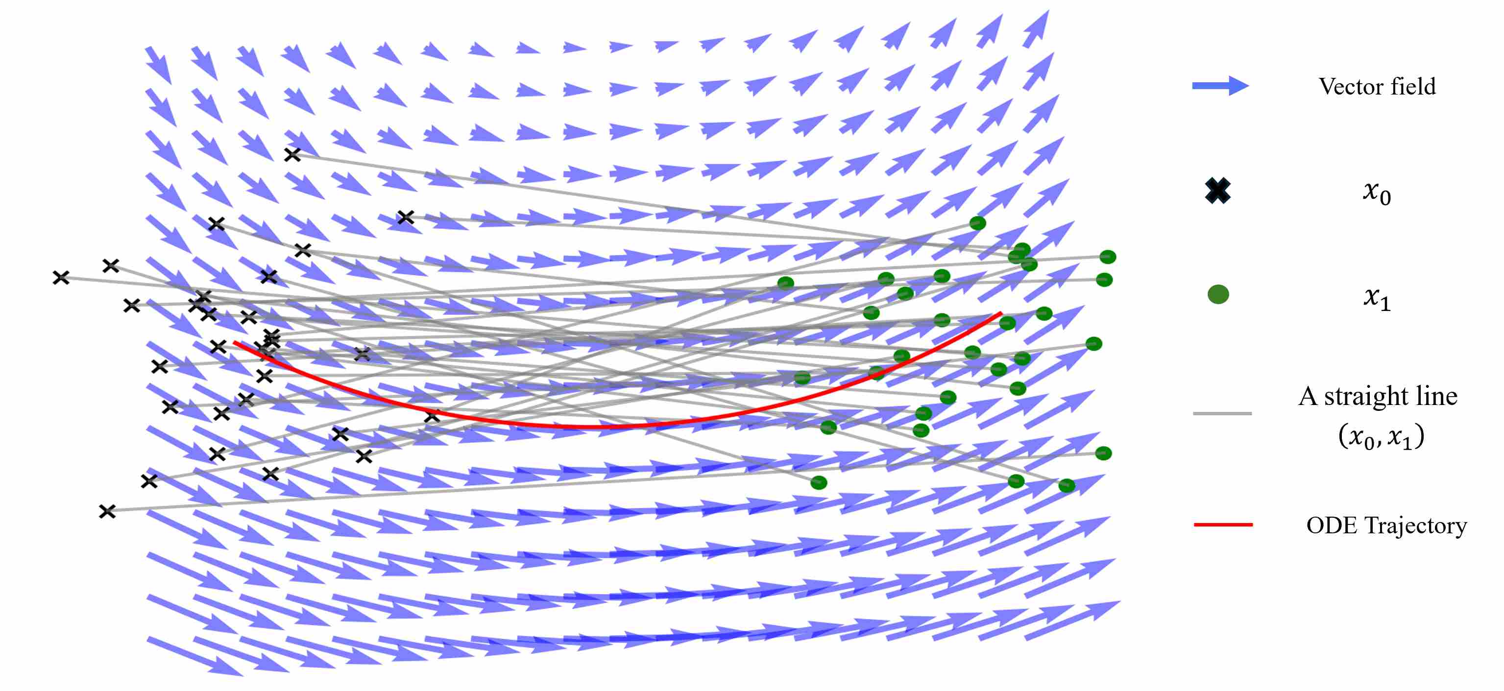
Flow Matching (FM) defines a straight path between a base distribution $p_0$ (e.g., Gaussian noise) and the data distribution $p_1$. In training, the target velocity field corresponds to the tangent of this straight line:

However, the model is only conditioned on $(t, x_t)$ and does not observe the specific pair $(x_0, x_1)$. As a result, the learned vector field is the marginal velocity field, i.e. the conditional expectation of all possible straight-line velocities passing through $x_t$.

Therefore, what the model learns is not the deterministic velocity of a specific straight-line path, but the conditional expectation of velocities across all possible paths at that point. This means even though the training objective enforces straight lines, the learned ODE trajectories $\tfrac{dx}{dt} = v_\theta(t,x)$ are generally curved.

This discrepancy motivates ReFlow (Rectified Flow): an iterative method to straighten the learned trajectories and accelerate sampling.

2.2.1 Implementation: How ReFlow Works

ReFlow ¹ is an iterative self-distillation procedure applied on top of FM:

1. Warmup with real endpoints

   • Train the model with real data samples $x_1 \sim p_{\text{data}}$.
   • This anchors the velocity field to the true data manifold.

2. Synthetic endpoints generation

   • Use the current (EMA) model as a teacher.
   • Sample from $p_0$ and integrate the learned ODE to obtain synthetic endpoints $\tilde{x}_1$.
   • These endpoints may be off-manifold or of imperfect quality.

3. Mixing strategy

   • Build a training buffer that contains both real endpoints and synthetic endpoints.
   • During training, each minibatch uses a mixture: with probability $1-p$ take a real endpoint, with probability $p$ take a synthetic endpoint.
   • The mixing ratio $p$ is gradually increased across rounds (e.g., from 0.4 → 0.9).

4. Rectification step

   • Regardless of whether the endpoint is real or synthetic, the teacher velocity is again defined as the straight-line velocity:

     \[u^{\star}(x_t) = \frac{x_1 - x_0}{1-t} \quad \text{(or equivalently } x_1 - x_0 \text{ for straight paths)}.\]

   • Thus the model is always forced to interpret the path as a straight line between the chosen endpoints.

5. Iteration

   • Repeat: generate new synthetic endpoints with the updated model, refill the buffer, retrain with mixing.
   • After a few rounds, the flow field becomes increasingly straightened.

2.2.2 Why ReFlow is Correct

A natural concern is: if synthetic endpoints are poor quality or off-manifold, wouldn’t the model drift further away from real data? ReFlow avoids this problem through two safeguards:

1. Real endpoints remain in training

   • Real data samples are always part of the mixture.
   • They serve as an anchor, preventing the flow field from collapsing onto low-quality synthetic samples.

2. Straight-path supervision is independent of endpoint quality

   • Even if a synthetic endpoint $\tilde{x}_1$ is imperfect, the loss still enforces a straight-line path between $x_0$ and $\tilde{x}_1$.
   • This “rectification” objective simplifies the geometry of the velocity field, making trajectories straighter, regardless of endpoint realism.

3. Self-distillation effect

   • Similar to knowledge distillation, the model learns from both ground-truth endpoints and its own outputs.
   • Over iterations, the velocity field becomes smoother and more consistent, which leads to improved sampling efficiency.

4. EMA teacher + gradual mixing

   • Using an exponential moving average (EMA) teacher to generate synthetic samples improves stability.
   • Gradually increasing the mixing ratio $p$ ensures the model does not overfit to poor synthetic samples in early rounds.

3. Model Distillation: Bypassing the ODE for One-Step Generation

While path linearization dramatically reduces the number of required steps by simplifying the ODE’s geometry, it still operates within the paradigm of numerical integration. Even a single-step Euler method on a rectified flow is fundamentally an approximation of an integral. Model distillation takes a more radical approach: it seeks to bypass the ODE solver entirely at inference time.

The core idea is to treat a pre-trained, multi-step generative model (the “teacher”) as a high-quality data generator. A new, compact model (the “student”) is then trained to replicate the teacher’s final output in a single forward pass. This reframes the generative task from a path integration problem into a direct function approximation problem, aiming to learn the ODE’s solution map directly.

In Essence: Instead of learning the velocity field $v(x, t)$ and integrating it, distillation learns the flow map $\Phi(x_0, 0, 1)$ that transports noise $x_0$ directly to the final sample $x_1$.

3.1 InstaFlow: A Case Study in Multi-Objective Distillation

A naive distillation using only pixel-wise loss (e.g., L2) would result in blurry, overly smoothed images, as the student would learn the average of the teacher’s potential outputs. InstaFlow provides a powerful blueprint for effective distillation by employing a multi-objective loss function that preserves detail and realism.

Given a noise vector $z$, we compute the student’s output $x_{\text{student}} = G_{\theta}(z)$ and the teacher’s reference output $x_{\text{teacher}} = M_{\text{teacher}}(z)$. The student is trained to minimize a weighted sum of three critical loss components:

1. Reconstruction Loss ($\mathcal{L}_{\text{rec}}$): A standard pixel-level loss, such as L1 or L2 distance, anchors the student’s output to the teacher’s global structure and color. \(\mathcal{L}_{\text{rec}} = \mathbb{E}_{z \sim p_0} \left[ \| G_{\theta}(z) - x_{\text{teacher}} \|_1 \right]\) While essential, this loss alone is insufficient for capturing high-frequency details.

2. Perceptual Loss ($\mathcal{L}_{\text{LPIPS}}$): To align the outputs with human perception, a perceptual loss like LPIPS is used. It measures the distance between the two images in a deep feature space (e.g., from a VGG network), penalizing textural and structural inconsistencies that pixel-wise losses ignore. \(\mathcal{L}_{\text{LPIPS}} = \mathbb{E}_{z \sim p_0} \left[ \text{LPIPS}(G_{\theta}(z), x_{\text{teacher}}) \right]\)

3. **Adversarial Loss ($\mathcal{L}{\text{adv}}$)**: This is the most critical component for achieving realism. A discriminator network $D$ is trained to distinguish between “real” samples from the teacher ($x{\text{teacher}}$) and “fake” samples from the student ($G_{\theta}(z)$). The student, in turn, is trained to fool the discriminator. This forces the student’s output distribution to match the teacher’s, effectively combating mode collapse and encouraging the generation of sharp, plausible details that might be statistically insignificant but are perceptually vital. \(\mathcal{L}_{\text{adv}} = \mathbb{E}_{z \sim p_0} \left[ -\log D(G_{\theta}(z)) \right]\)

The final objective is a weighted combination: \(\mathcal{L}_{\text{total}} = \lambda_{\text{rec}}\mathcal{L}_{\text{rec}} + \lambda_{\text{LPIPS}}\mathcal{L}_{\text{LPIPS}} + \lambda_{\text{adv}}\mathcal{L}_{\text{adv}}\)

This multi-objective approach ensures the student not only matches the content of the teacher’s output but also its stylistic and distributional properties, leading to high-quality one-step generation.

8. References