A General Discussion of Flow Matching

Flow matching ¹² is a continuous-time generative framework in which you learn a time-dependent vector field $v_{\theta}$, whose flow transports samples from a simple prior distribution ( usually a standard gaussian distribution) at $t=0$ to your target data distribution at $t=1$.

preliminaries

In this section, we first summarize the key terms and terminology needed for learning flow matching.

Vector Field: vector field is a function that assigns to each spatial point $x_t \in \mathbb R^d$ and time $t \in [0, 1]$ an instantaneous velocity $v_{\theta}(t, x_t)$:

ODE: ODE (Ordinary Differential Equation) is the dynamical law you impose using that vector field:

Solving this ODE from $t=0$ to $t=1$ is equivalent to sampling, whose goal is to transport an initial point $x_0$ to a target $x_1$ through space according to the learned velocities.

Trajectory: A trajectory $(x_0, \dots, x_{t}, \dots,x_1)$, is simply the solution of the above ODE for a given start point $x_0$. It’s the continuous path that the “particle” traces out under the influence of the vector field:

Or using the Euler method to solve in a discrete time step:

Flow: a flow is essentially a collection of trajectories that follows the ODE, that means by solving the above ODE we gather a lot of solutions for different initial points

Probability path

The first step of FM is to define a probability path, who specifies a gradual interpolation from initial distribution $p_{init}$ to target distribution $p_{data}$.

Conditional probability path: given an end point $z \sim p_{data}$, a conditional probability path is the distribution of an intermediate sample conditioned on $z$, denoted as $p_t(x_t|z)$ such that

Marginal probability path: marginal probability path defined as the distribution that we obtain by first sampling a data point $z ∼ p_{data}$ from the data distribution and then sampling from $p_t(x_t |z)$, we can formalize it as:

$p_t(x_t)$ satisfy $p_0(\cdot)=p_{init}$ and $p_1(\cdot)=p_{data}$. The difference between the marginal probability path and the conditional probability path can be illustrated as follows.

One particularly popular probability path is the Gaussian probability path.

Training Target

Our goal is to train a neural network $u_t^{\theta}(x_t)$ to approximate the true vector field, we accomplish this by minimizing a MSE loss function:

To solve this loss function, we need to calculate the target value $u_t(x_t)$. Equipped with a probability path $p_t(x_t)$, we can build a target vector filed $u_t(x_t)$, such that the corresponding ODE yield the probability path. given marginal probability path $p_t(x_t)$, then the marginal vector field $u_t(x_t)$ defined by

However, it is hard to compute $u_t(x_t)$ because the above integral is intractabl. Instead, we will exploit the conditional velocity field and modify the loss function from $\mathcal L_{FM}$ to $\mathcal L_{CFM}$:

conditional velocity field is tractabl, which makes it feasible to minimize $\mathcal L_{CFM}(\theta)$ mathematically. Given conditional probability path $p_t(x_t|z)$, then the conditional vector field $u_t(x_t|z)$ defined by

The marginal vector field can be viewd as averaging the conditional velocity fields $ut(x|x1)$ across targets, i.e.,

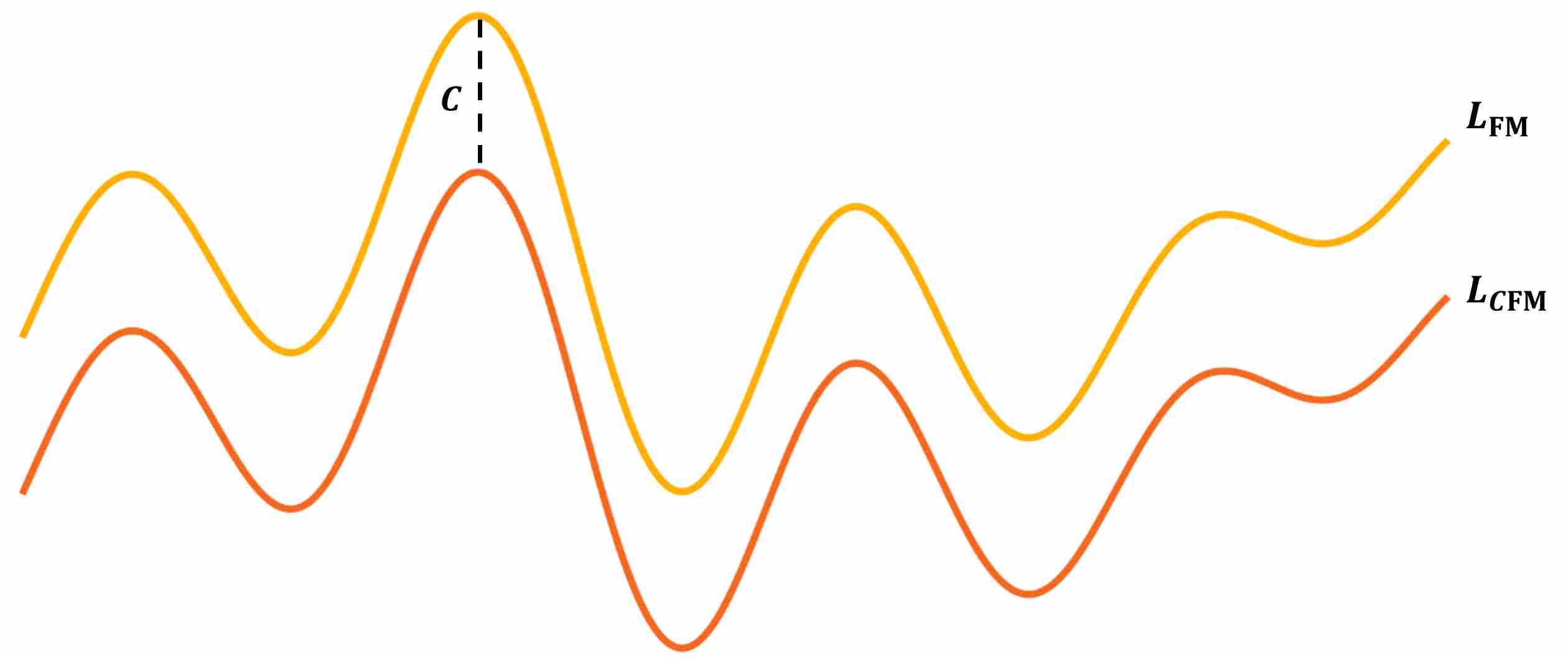
The key point is that $\mathcal L_{FM} = \mathcal L_{CFM}+C$, where $C$ is a constant, which means that minimizing $\mathcal L_{FM}$ is equal to minimizing $\mathcal L_{CFM}$ with represpect to $\theta$.

Consider the second term:

Now, Let’s substitute the second item with the result above:

We can summarize the relationship between $\mathcal L_{FM}$ and \mathcal L_{CFM} with the following figure.

References