
Controlled Generation with Diffusion Models
Published:
📚 Table of Contents
- 1. Introduction: From Unconditional to Controllable Generation
- 2. Steering the Diffusion Process with Global Guidance
- 3. Image Inversion
- 4. Latent and Semantic Control
- 5. Personalized Control: Injecting New Concepts into Diffusion Models
- 6. Structured Condition Control
- 7. Advanced Paradigms: Hybrid and Multimodal Controls
- 8. References
Diffusion models have emerged as a dominant paradigm for high-fidelity image synthesis, yet their native formulation remains largely uncontrolled, relying on stochastic sampling from an unconditional generative process. As real-world applications increasingly demand specificity, consistency, and interpretability, the field has rapidly evolved toward controllable diffusion generation—a unified framework for steering the sampling trajectory according to external conditions, semantic concepts, or structural priors.
In the previous articles, we have explored various aspects of knowledge related to diffusion models, covering their theoretical foundations, core algorithms, and architectural designs, as well as the training stability and efficiency. However, all the generation methods we discussed earlier are unconditional generation. This post provides a comprehensive analysis of controllable generation from a unified theoretical and architectural perspective.
1. Introduction
Current research on controllable diffusion models can be systematically organized into three major categories, defined by where and how the control signal interacts with the diffusion process.
Category 1: Guidance-based Control. This type of technology does not modify the model itself nor learn new knowledge. During inference, it adjusts the generation direction through algorithms to enhance the model’s adherence to existing instructions (primarily text prompts).
Category 2: Finetuning-based Control. This type of technology injects new, personalized knowledge into the model—such as specific faces, objects, or artistic styles—by finetuning part or all of the model’s parameters.
Category 3: Structure-based Control. This type of technology represents a major revolution in the field of controllable generation. Instead of relying on ambiguous text, it precisely controls the composition, layout, and structure of the generated image by providing explicit, pixel-level spatial information (such as skeletal poses, depth maps, edge maps, etc.).
Specifically, Guidance-based Control can be further divided into Global and Local (Semantic) subtypes, we summarize and compare these three Principal categories of Controllable Diffusion Models as follows.
| Category | Subtype / Control Level | Representative Methods | Model Modified | Learns New Knowledge | Control Scope | Description |
|---|---|---|---|---|---|---|
| 1. Guidance-based Control | (a) Global Guidance | Classifier Guidance, Classifier-Free Guidance | ❌ No | ❌ No | Global | Steers the overall sampling trajectory by adjusting score or noise predictions across all time steps. |
| (b) Local / Semantic Guidance | Attention Control, Prompt-to-Prompt, Null-Text Optimization, DiffEdit, EDICT | ❌ No | ❌ No | Local / Semantic | Modifies intermediate latent or attention representations to achieve localized, interpretable control. | |
| 2. Model Personalization | Parameter-level Control | LoRA, DreamBooth, Textual Inversion, Custom Diffusion | ✅ Yes | ✅ Yes | Instance / Concept | Fine-tunes part or all of the model to inject new, personalized or domain-specific knowledge. |
| 3. Structured Condition Control | Input-level Control | ControlNet, T2I-Adapter, IP-Adapter, SDEdit | ❌ No | ❌ No | Spatial / Structural | Incorporates explicit spatial conditions (pose, depth, edge, segmentation) to control composition and layout. |
Finally, we discuss emerging trends including compositional and multimodal control, it is not a fundamentally new mechanism. Rather, it extends the above three paradigms to multi-signal or multi-modal conditioning — for example, combining text + pose (ControlNet), text + image exemplar (IP-Adapter), or text + video + audio (AnimateDiff, VideoFusion). It operates as a compositional layer across the three categories, not a standalone paradigm.
2. Steering the Diffusion Process with Global Guidance
Diffusion models were originally designed as unconditional generators that progressively denoise Gaussian noise to recover clean data samples. In many real applications, however, users desire to steer the generation toward specific conditions—text prompts, categories, objects, or visual attributes—without retraining the model. Inference-time guidance methods accomplish exactly this: they introduce an external “force field” that modifies the sampling trajectory so that the generated sample follows the direction favored by a given condition $c$. The model itself remains fixed; only the sampling dynamics are altered.
2.1 A Unified Principle for Global Guidance
Goal. We want to steer a fixed diffusion model at inference time — without retraining — so that the generated sample $x_0$ better matches a user condition $c$ (text, class label, image cue, etc.). All methods in this family can be seen as injecting a condition-dependent force field into the reverse denoising dynamics. Recall the reverse-time sampler (SDE or ODE) of the unconditional model be
\[\mathrm{d}x_t =\Big[f(t)x_t - g^2(t)\nabla_{x_t}\log p_t(x_t)\Big]\mathrm{d}t + g(t)\,\mathrm{d}\bar w_t,\]where $p_t(x_t)$ is the marginal density at time $t$. Replacing the unconditional score by the conditional one yields:
\[\mathrm{d}x_t =\Big[f(t)x_t - g^2(t)\nabla_{x_t}\log p_t(x_t \mid c)\Big]\mathrm{d}t + g(t)\,\mathrm{d}\bar w_t,\]where $c$ is condition signal. By Bayes’ rule, the conditional score can be decomposed into two components.
\[\nabla_{x_t}\log p(x_t \mid c) = \nabla_{x_t}\log p(c \mid x_t) \;+\; \nabla_{x_t}\log p(x_t)\label{eq:score_based_lens}\]Replacing the conditional score and yields:
\[\mathrm{d}x_t=\Big[f(t)x_t - g^2(t)\underbrace{\nabla_{x_t}\log p_t(x_t)}_{\text{unconditional score}} - g^2(t)\underbrace{\nabla_{x_t}\log p_t(c \mid x_t)}_{\text{classifier gradient}} \Big]\mathrm{d}t + g(t)\,\mathrm{d}\bar w_t\label{eq:cg}\]This equation shows that conditional generation can be achieved by adding a drift term proportional to $\nabla_{x_t}\log p(c\mid x_t)$—an external force directing samples toward class $c$. Different guidance families differ only in how they approximate the guidance direction term.
Equation \ref{eq:score_based_lens} is derived from the perspective of score prediction; in fact, we can generalize this conclusion to other objectives: For all four common parameterizations—$\epsilon$-prediction, $v$-prediction, score-prediction, and $x_0$-prediction — guidance reduces to the same mixing rule :
\[g_{\text{total}} \;=\; g_{\text{uncond}} \;+\; w\,g_{\text{guide}}, \qquad g\in{\epsilon,\,v,\,s,\,x_0}.\]For the convenience of discussion, we will base all subsequent discussions on $\epsilon$-prediction.
2.2 Classifier Guidance
Classifier Guidance 1 was the first practical approach to achieve controllable generation in diffusion models without retraining the generative model itself. It introduces an external classifier to steer the diffusion sampling process toward samples consistent with a target condition—typically a class label $c$.
Since $p(y\mid x_t)$ is unknown, an auxiliary noisy-image classifier $p_\phi(y\mid x_t, t)$ is trained on images corrupted with the same diffusion noise. Its gradient approximates the desired term:
\[\nabla_{x_t}\log p(c \mid x_t) \;\approx\; \nabla_{x_t}\log p_\phi(c \mid x_t)\]This is why it is called classifier guidance. Substituting into \ref{eq:cg} gives the classifier-guided reverse SDE:
\[\mathrm{d}x_t=\Big[f(t)x_t - g^2(t)\nabla_{x_t}\log p_t(x_t) - s(t)\nabla_{x_t}\log p_\phi(c\mid x_t) \Big]\mathrm{d}t + g(t)\,\mathrm{d}\bar w_t,\]where $s(t)$ controls the guidance strength (often increasing as noise decreases). The classifier gradient can be efficiently obtained by backpropagating through the classifier with respect to its input $x_t$.
Summary: Classifier Guidance marked the first practical demonstration that diffusion trajectories can be steered at inference time by introducing an external gradient field derived from a classifier. Its theoretical contribution was fundamental: it established the now-standard view that conditional generation equals unconditional generation plus a conditional gradient term. However, the approach suffers from several inherent limitations:
Firstly, it requires training an additional classifier on noisy images for every diffusion timestep, incurs substantial computational cost due to per-step backpropagation.
Secondly, and most critically, it offers control only over discrete semantic categories rather than fine-grained attributes or spatial structures.
As a result, its applicability remains narrow and inefficient for complex or continuous conditions. Nevertheless, Classifier Guidance’s conceptual insight directly inspired subsequent advances such as Classifier-Free Guidance, Attention-based Control, and ControlNet, which internalized or generalized the same principle into far more flexible and efficient conditioning mechanisms.
2.3 Classifier-Free Guidance (CFG)
Classifier-Free Guidance 2 is the most widely used inference-time guidance method in modern diffusion systems (e.g., Stable Diffusion, Imagen, SDXL). It internalizes the conditional gradient used by Classifier Guidance, but removes the external classifier: during training, the same denoiser learns both conditional and unconditional predictions. At inference, we combine these two predictions to emulate ascent on the conditional likelihood—recovering the unified “external force” view while keeping the model frozen.
Training setup: Let $c$ denote conditioning (text, label, etc.). During training, with probability $p_{\text{drop}}$ we replace $c$ by a special null token $\varnothing$. The standard denoising loss is
\[\min_\theta\;\mathbb{E}_{x_0,c,t,\epsilon} \Big\|\epsilon - \epsilon_\theta(x_t,\tilde c,t)\Big\|^2, \quad \tilde c=\begin{cases} c & \text{w.p. } 1-p_{\text{drop}},\\ \\ \varnothing & \text{w.p. } p_{\text{drop}}. \end{cases}\]Thus the same network learns two behaviors: Conditional branch: $\epsilon_\theta(x_t,c,t)$, and Unconditional branch: $\epsilon_\theta(x_t,\varnothing,t)$.
This duality is the key to estimating $\nabla_{x_t}\log p(c\mid x_t)$ without a classifier. By Bayes,
\[\begin{align} \nabla_{x_t}\log p(c\mid x_t) & =\nabla_{x_t}\log p(x_t\mid c)-\nabla_{x_t}\log p(x_t) \\[10pt] & \approx -\frac{1}{\sigma_t}\Big(\epsilon_\theta(x_t,c,t)-\epsilon_\theta(x_t,\varnothing,t)\Big) \end{align}\]This means CFG replaces the external estimator with an internal contrast between the model’s conditional and unconditional predictions.
\[{\epsilon}_{\text{guide}} = {\epsilon}_{\text{cond}} - {\epsilon}_{\text{uncond}}\]Plug this approximation into the unified dynamics and absorb constants into $\lambda(t)$. In discrete sampling (DDPM/DDIM/ODE), this becomes the familiar guided denoiser:
\[\begin{align} {\epsilon}_{\text{total}} & = {\epsilon}_{\text{uncond}} + w(t)\cdot{\epsilon}_{\text{guide}} = {\epsilon}_{\text{uncond}} + w(t)\cdot\left( {\epsilon}_{\text{cond}} - {\epsilon}_{\text{uncond}} \right) \\[10pt] & =\epsilon_\theta(x_t,\varnothing,t) + w(t)\cdot\left(\epsilon_\theta(x_t,c,t)\;-\epsilon_\theta(x_t,\varnothing,t) \right) \\[10pt] & = w(t)\cdot\epsilon_\theta(x_t,c,t) + (1-w(t)) \cdot\epsilon_\theta(x_t,\varnothing,t) \end{align}\]where $w(t)\ge 0$ is the guidance scale. Large $w$ increases faithfulness to $c$ (mode-seeking), small $w$ preserves diversity (mode-covering).
Summary: Classifier-Free Guidance (CFG) represents a pivotal evolution of the inference-time guidance paradigm first introduced by Classifier Guidance (CG).
- CFG eliminates the need for a noisy-image classifier, drastically reducing computational and training cost.
- It also generalizes beyond discrete categories, allowing conditions to be continuous, multimodal, or high-dimensional (e.g., text embeddings, style vectors).
- It also generalizes beyond discrete categories, allowing conditions to be continuous, multimodal, or high-dimensional (e.g., text embeddings, style vectors).
For this reason, CFG became the standard backbone of controllable diffusion systems such as Stable Diffusion, Imagen, and SDXL.
2.4 Multi-Condition Guidance in Diffusion Models
In practice, Conditional diffusion models are rarely driven by a single signal in practice. Real deployments combine heterogeneous condition types (channels)—e.g., Text, Layout/Boxes, Segmentation, Depth/Normals, Reference Image/Style—to control complementary aspects of content and geometry. Moreover, conditions may be positive (encouraging the presence of attributes) or negative (suppressing undesired content). These signals can be statistically independent, weakly dependent, or directly conflicting (e.g., a style that clashes with layout geometry).
In previous section, we discuss the classical guidance mechanisms (e.g., classifier guidance (CG) and classifier-free guidance (CFG)) with single condition. Extending them systematically to multiple, potentially competing conditions requires a careful treatment of the following questions:
How to train with multiple channels, this is crucial for the guidance sampling with multiple conditions.
How to combine multi-condition at inference, and get the final guidance directions.
Handling dependencies and conflicts across channels, including priority and scheduling.
Definition (Channel): A channel is a condition type with its own encoder and null state (e.g., text tokens and a text-null token; depth image and a "depth-off" code).
Key clarification: Multi-condition refers to multiple condition types/channels, not the count of inputs within a type. One hundred sentences still constitute one text channel; one depth map per target image constitutes one depth channel. When desired, a single channel (e.g., text) may be factorized into sub-conditions for finer control, but it remains one modality/channel.
2.4.1 Problem Setup and Notation
Let $x_0\sim p_{\text{data}}$, and $x_t=\alpha(t)x_0+\sigma(t)\epsilon$ be a VP-type forward process. Let channels
\[\mathcal{K}=\{\text{text},\text{layout},\text{seg},\text{depth},\text{normal},\text{ref},\dots\}\]For channel $k\in\mathcal{K}$, denote its input by $c_k$ as positive conditions, $c^-_k$ as negative conditions and its channel-specific null by $\varnothing^{(k)}$. Formally, we can uniformly represent the set of multiple conditions as
\[\mathcal{C}\;=\;\{c_1,\ldots,c_K\}\;\cup\;\{c^-_1,\ldots,c^-_K\}\]where $c_k$ are positive conditions to be promoted and $c^-_m$ are negative conditions to be suppressed. The unconditional probability-flow ODE is
\[\frac{dx_t}{dt}=f_\theta(x_t,t).\]Guidance augments the drift by a vector field
\[\frac{dx_t}{dt}=f_\theta(x_t,t)+\lambda(t),g(x_t,t), \quad g(x_t,t)=\nabla_{x_t}\log p(\mathcal{C}\mid x_t),\]We adopt $\epsilon$-prediction for exposition; formulas transpose to $x_0$ and $v$-prediction.
2.4.2 Training with Multiple Channels: Per-Channel Dropout
Training must align the model with all subsets of channels it may face at inference. We therefore use independent per-channel dropout (a.k.a. classifier-free dropout per channel).
To this end, we define Sampling masks For each channel $k$, draw a keep mask
\[m_k\sim\mathrm{Bernoulli}\,\big(k_k(t)\big),\quad k_k(t)=1-q_k(t),\]and form the training input
\[\tilde c_k=\begin{cases} c_k & \text{if } m_k=1\ \text{and channel is available},\\ \\ \varnothing_k & \text{otherwise}. \end{cases}\]The loss (for $\epsilon$-prediction) is
\[\mathcal{L}=\mathbb{E}_{x_0,t,\epsilon}\ \mathbb{E}_\ \big\|\epsilon-\epsilon_\theta\big(x_t,\,t;\tilde c_1,\ldots,\tilde c_{|\mathcal{K}|}\big)\big\|_2^2.\]Unconditional frequency. If a target unconditional rate (u\in[0.1,0.2]) is desired,
\[\Pr\{\text{all dropped}\}=\prod_{k} q_k(t)\approx u,\]e.g., with equal rates $q_k=q$ one can set $q=u^{1/|\mathcal{K}|}$. Optionally use SNR/$\sigma$-aware $q_k(t)$ (higher dropout at high noise).
Implementation essentials: Each channel must have its own null embedding . There is no “negative condition” in training; negative guidance only exists in inference.
2.4.3 Inference: Channel-Wise Guidance and Composition
We consider a set of conditions consists of positive conditions $\mathcal{P}$ and negative conditions $\mathcal{N}$
\[\mathcal{C} \;=\; \underbrace{\{c_1,\ldots,c_K\}}_{\text{positive conditions} \mathcal{P}} \;\cup\; \underbrace{\{c^-_1,\ldots,c^-_M\}}_{\text{negative conditions} \mathcal{N}}\]where $c_k$ are positive conditions to be promoted and $c^-_m$ are negative conditions to be suppressed. Assume the conditions are conditionally independent given $x_t$. Using a first-order sum-of-experts surrogate,
\[\nabla_{x_t}\log p_t(\mathcal{C} \mid x_t) \;\approx\;\sum_{k=1}^K\nabla_{x_t}\log p_t(c_k\mid x_t)\;-\;\sum_{m=1}^M\nabla_{x_t}\log p_t(c^-_m\mid x_t).\]At inference we form channel-wise conditional–unconditional differences and linearly compose them. Let
\[\epsilon_u=\epsilon_\theta(x_t,t;\ \forall k:\ \varnothing^{(k)}),\quad \epsilon_{k}=\epsilon_\theta\big(x_t,t;\ c^{(k)}\text{ on},\ \text{others as configured}\big).\]A simple and robust choice is to define the per-channel difference
\[d_k=\epsilon_{k}-\epsilon_u,\]and the guided prediction
\[\epsilon_{\text{total}} =\epsilon_u+\underbrace{\sum_{k\in\mathcal{P}} w_k(t)\,d_k}_{\text{positive guide}} \;-\; \underbrace{\sum_{k\in\mathcal{N}} w_k^-(t)\,d_k}_{\text{negative guide}}\]for positive channels $\mathcal{P}$ and negative channels $\mathcal{N}$ (negative prompts use negative weights). Plug $\epsilon_{\text{total}}$ into any sampler (DDIM, Heun/RK, DPM-Solver, …). SNR/(\sigma)-aware scheduling. Use (w_k(t)=\bar w_k\cdot\mathrm{SNR}(t)^{\alpha_s}) or (w_k(\sigma)=\bar w_k\cdot \sigma^{-\beta}) to weaken guidance at high noise and avoid late oversharpening (typical (\alpha_s,\beta\in[0.3,0.7])).
Note. If a single channel (e.g., text) is deliberately split into “sub-prompts”, (1) still applies with the sub-prompts indexed by (k). This is a within-channel factorization for finer control, not a new modality.
3. Image Inversion
Prompt-to-Prompt (P2P) enables semantic-level editing by replacing or interpolating specific columns in the cross-attention maps between a source prompt $c_s$ and a target prompt $c_t$, while keeping other parts of the scene intact. During sampling, both prompts are processed under the same noise initialization $x_T$, and the attention maps are fused step-by-step to ensure that unchanged tokens preserve their original spatial correspondences.
However, this mechanism assumes the availability of the initial noise $x_T$, which is only known for synthetic images generated by the diffusion model itself. In real-world applications, we start from a given real image $x_0$ instead of a noise latent, and thus cannot directly apply P2P. Consequently, a central research problem has emerged:
How can we map a real image $ x_0 $ into the latent space of a pre-trained diffusion model so that it can be faithfully reconstructed and semantically edited like a generated image?
This challenge—known as diffusion inversion—aims to find a noise latent $ x_T $ (and potentially auxiliary parameters) such that the forward diffusion trajectory under the model’s learned dynamics reproduces the given real image.
3.1 Null-Text Inversion (NTI)
NTI 3 is the most widely adopted optimization-based approach. It proceeds in two stages:
Stage I: Pivotal inversion. We first construct a stable reference (pivot) trajectory \(\{x_t^\star\}_{t=0}^{T}\) by inverting $x_0$ with a guidance-neutral setting (guidance scale $w=1$). Concretely, for DDIM with \(\bar\alpha_t=\prod_{s=1}^t(1-\beta_s)\) and $\eta=0$ (deterministic ODE limit), define the denoiser used in inversion as
\[\widehat\epsilon_t^{\text{inv}} \,=\, \epsilon_\theta\,\big(x_t^\star,\,t,\,c\big) \quad (\text{equivalently CFG with }w{=}1).\]One inversion step $t \to t{+}1$ is
\[x_{t+1}^\star = \sqrt{\bar\alpha_{t+1}}\;\hat x_0^{(t)} \;+\; \sqrt{1-\bar\alpha_{t+1}}\;\widehat\epsilon_t^{\text{inv}}\]where
\[\hat x_0^{(t)} = \frac{x_t^\star - \sqrt{1-\bar\alpha_t}\,\widehat\epsilon_t^{\text{inv}}}{\sqrt{\bar\alpha_t}}\]Initialization sets \(x_0^\star \,=\, \text{Encoder}(x_0)\) for latent diffusion, or $x_0^\star = x_0$ for pixel diffusion. Iterating \(t=0\!\to\!T{-}1\) yields the pivotal latent $x_T^\star$ and the full reference path.
Why $w{=}1$ here? Large guidance scalars nonlinearly amplify modeling/rounding errors and make the inverse ODE numerically fragile. Using (w{=}1) produces a smooth, model-consistent path that is easier to “close” in Stage II.
Stage II: Null-Text Optimization. Because DDIM inversion relies on the model’s imperfect noise prediction and a discretized deterministic ODE, the forward (inversion) and backward (sampling) trajectories are not mathematically identical. Small approximation errors in $\epsilon_\theta(x_t,t,c)$, guidance nonlinearity (CFG), and numerical discretization accumulate over timesteps, causing the reconstructed image $\hat{x}_0$ to deviate slightly from the original $x_0$.
NTI fixes this without changing network weights by optimizing the null (unconditional) embeddings ${\mathcal O_t}$ (one per step), keeping the conditional prompt embedding $c$ frozen. With CFG, the denoiser is
\[\epsilon_{\text{total}}(x_t,t;\mathcal O_t)\;=\; \epsilon_\theta(x_t,t,\mathcal O_t)\;+\;w\!\left(\epsilon_\theta(x_t,t,c)\;-\;\epsilon_\theta(x_t,t,\mathcal O_t)\right).\]Given a current state $x_t$, the DDIM one-step predictor with \(\eta\!=\!0\) is
\[x_{t-1}\,\leftarrow\,\operatorname{DDIMstep}(x_t;\mathcal O_t) = \sqrt{\bar\alpha_{t-1}}\;\widehat x_0^{(t)}(\mathcal O_t) + \sqrt{1-\bar\alpha_{t-1}}\;\epsilon_{\text{total}}\]where
\[\widehat x_0^{(t)}(\mathcal O_t) \;=\; \frac{x_t - \sqrt{1-\bar\alpha_t}\,\epsilon_{\text{total}}}{\sqrt{\bar\alpha_t}}\]
In this way, the path inversion problem is reduced to an optimization problem. Its goal is to find the optimal null text embedding $(\mathcal O_t)$, that aligns the forward pivotal trajectories and backward paths for any time step $t$. Total objective is
\[\boxed{ \min_; \mathcal L_{\text{NTI}} \;=\; \mathcal L_{\text{rec}} \;+\; \mathcal L_{\text{smooth}} \;+\; \mathcal L_{\text{img}} }\]where $\mathcal L_{\text{rec}}$ represents reconstruction loss, which enforces the reference-path consistency:
\[\mathcal L_{\text{rec}}({\mathcal O_t}) \;=\; \sum_{t=1}^{T} \Big\|\,\operatorname{DDIMstep}(x_t^\star;\mathcal O_t) \;-\; x_{t-1}^\star \Big\|_2^{2}.\]$\mathcal L_{\text{smooth}}$ represents Temporal smoothness, which avoid step-wise jitter and improve stability:
\[\mathcal L_{\text{smooth}}({\mathcal O_t}) \;=\; \lambda \sum_{t=2}^{T}\big\|\,\mathcal O_t - \mathcal O_{t-1}\,\big\|_2^{2}.\]$\mathcal L_{\text{img}}$ represents Pixel-/Perceptual-space nudges, which should be kept small to avoid leaking information outside the diffusion dynamics. After decoding $ \widehat x_0 \,=\, \text{Decoder}(\widehat x_0^{\star})$ from the last step, one may add
\[\mathcal L_{\text{img}} \;=\; \mu_1\,\|\widehat x_0 - x_0\|_1 \;+\; \mu_2\,\text{LPIPS}(\widehat x_0, x_0)\]We optimize ${\mathcal O_t}_{t=1}^{T}$ by back-propagating through the DDIM steps with the network frozen (tens of iterations suffice). The result is a closed guided trajectory: starting from $x_T^\star$ and using $(c,{\mathcal O_t^\star},w)$, the sampler reconstructs $x_0$ almost exactly.
3.2 Negative-Prompt Inversion (NPI)
While Null-Text Inversion (NTI) achieves highly faithful reconstructions by iteratively optimizing the null-text embeddings, its step-wise optimization introduces significant computational overhead. To address this limitation, Negative-Prompt Inversion (NPI) 4 proposes a zero-optimization alternative that approximates NTI’s behavior through an elegant reinterpretation of the classifier-free guidance (CFG) framework.
In NTI, the optimized null-text embeddings $\emptyset_t^\star$ are found to gradually converge toward the conditional embedding $c$ as the optimization proceeds. This empirical observation suggests that the “optimal” unconditional branch in CFG is not necessarily an empty string, but a semantically meaningful embedding closely aligned with the prompt itself. Motivated by this, NPI directly replaces the null-text embedding with the conditional embedding, i.e.,
\[\emptyset_t = c,\]thus eliminating the need for per-step optimization while retaining the structural advantages of NTI. Recall the standard classifier-free guidance:
\[\begin{align} \epsilon_{\text{CFG}}(x_t, t, c, \emptyset_t) = \epsilon_\theta(x_t, t, \emptyset_t) + w \big( \epsilon_\theta(x_t, t, C) - \epsilon_\theta(x_t, t, \emptyset_t) \big) \\[10pt] & = \epsilon_\theta(x_t, t, c) \end{align}\]Once the inversion step produces (x_T), the same latent code can be used with Prompt-to-Prompt (P2P) editing. During sampling, P2P manipulates the cross-attention maps by replacing or fusing token-specific attention between the source and edited prompts, while NPI provides a consistent unconditional embedding $(C_\text{src})$ for CFG-based guidance. The combination yields efficient and structurally consistent editing:
\[\begin{align} \epsilon_{\text{CFG}}(x_t, t, C_\text{tar}, C_\text{src}) & = \epsilon_\theta(x_t, t, \emptyset) + w \big( \epsilon_\theta(x_t, t, C_\text{edit}) - \epsilon_\theta(x_t, t, \emptyset) \big) \\[10pt] & = \epsilon_\theta(x_t, t, C_\text{src}) + w \big( \epsilon_\theta(x_t, t, C_\text{edit}) - \epsilon_\theta(x_t, t, C_\text{src}) \big) \end{align}\]It is observed that during subsequent editing with NPI, the null prompt $(\emptyset)$ needs to be replaced with source prompt $(C_{\text{src}})$, making the source prompt acts like a negative prompt, and this is how the name “NPI” originates.
3.3 EDICT
3.4 BDIA
4. Local Guidance: Latent and Semantic Control
While global guidance methods like CFG are remarkably effective at strengthening the alignment between a generated image and its condition, the guidance scale w amplifies the conditional signal across the entire image, pushing the whole generation trajectory in a uniform direction. This approach lacks the finesse needed for region-specific edits, object-level manipulation, or preserving the layout of an image while changing its content.
To overcome these limitations, a new family of methods emerged: Local or Semantic Guidance. Instead of modifying the final output vector, local/semantic control intervenes inside the diffusion trajectory—on selected tokens, spatial regions, or intermediate features—so edits are localized and interpretable (e.g., “cat→dog” without touching background). The model remains frozen; we alter the representations it manipulates.
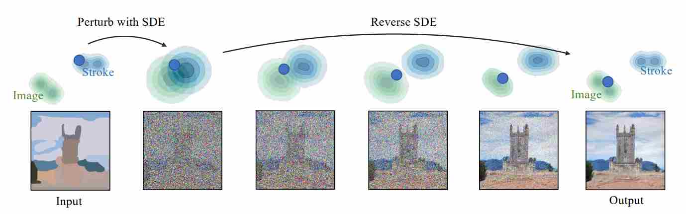
4.1 SDEdit: Structure-Preserving Editing via Stochastic Denoising
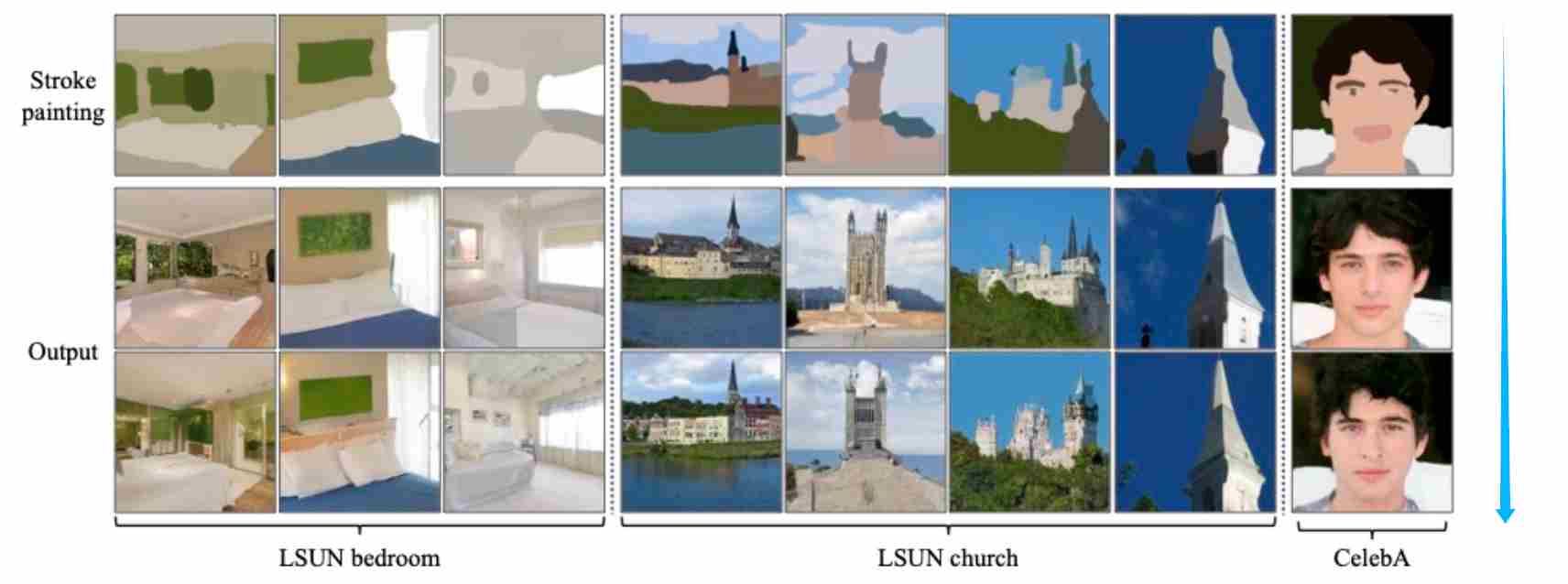
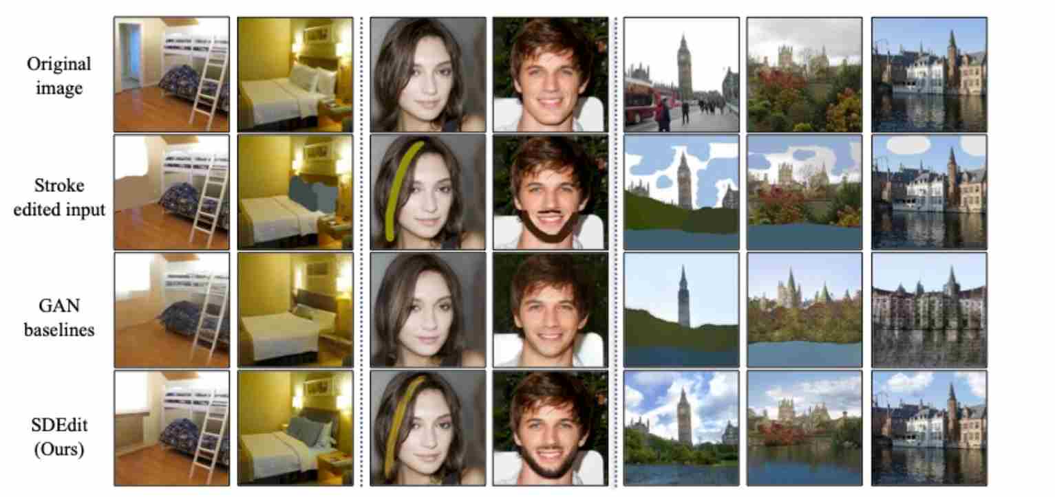
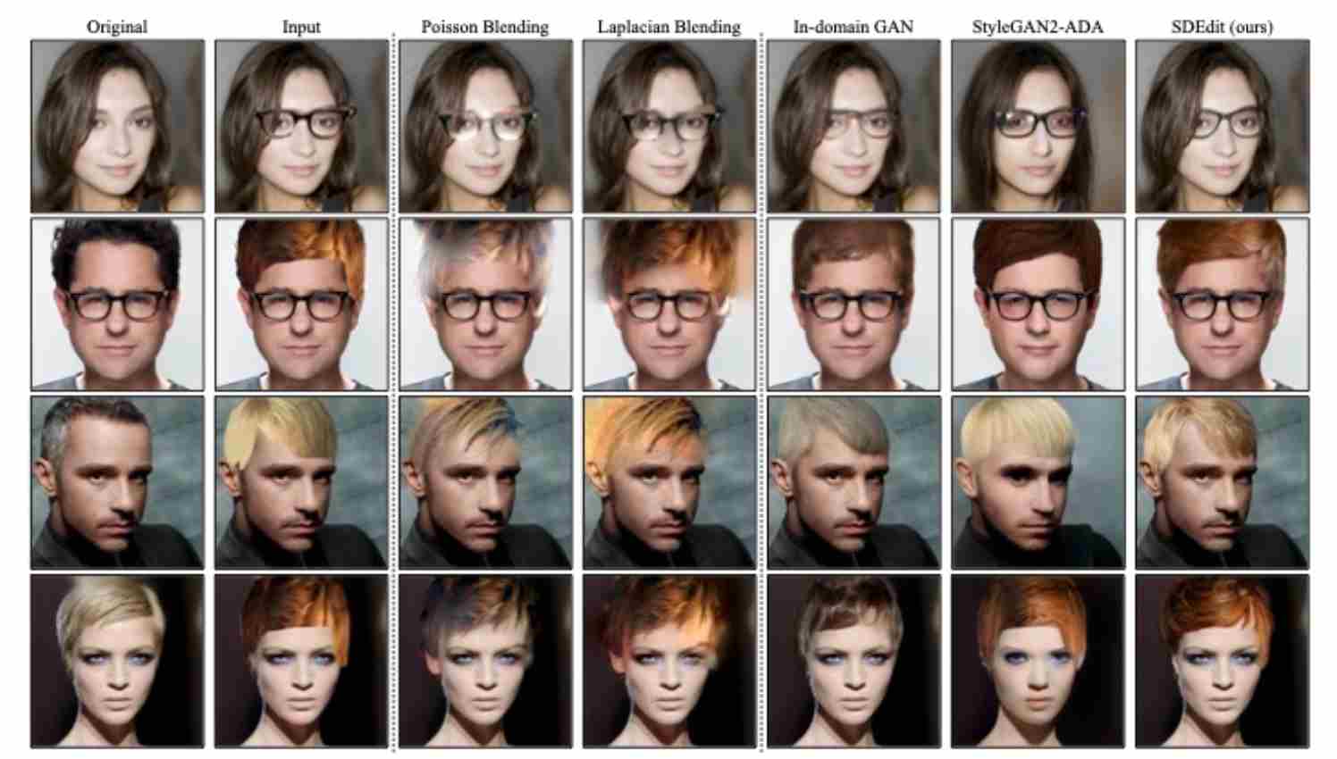
SDEdit 5 (short for Stochastic Differential Editing) enables structure-preserving image translation—turning coarse sketches, partial paintings, or corrupted photos into realistic outputs—without retraining the diffusion model.
Instead of conditioning generation on textual semantics, SDEdit controls the structural layout of the image through the initial state of the reverse diffusion process, as illustrated in the figure below. Given an input image $x_0^{\text{in}}$ (e.g., a line drawing, depth map, or degraded photo), SDEdit first adds Gaussian noise until a moderate noise level $t_0$ and then runs the reverse SDE/ODE from $t_0 \to 0$ using a pretrained denoiser. The result $x_0^{\text{out}}$ retains the large-scale composition of $x_0^{\text{in}}$ while restoring fine details and realism
Typical applications include:
Case 1: Synthesizing images from strokes. Given an input stroke painting, our goal is to generate a realistic image that shares the same structure as the input when no paired data is available.
Case 2: Stroke-based local editing. Given an input with user added strokes, we want to generate a realistic image based on the user’s edit.
Case 3: Image compositing with SDEdit. Given an image, users can specify how they want the edited image to look like using pixel patches copied from other reference images.
Crucially, SDEdit requires no textual prompt; its control arises entirely from the visual structure embedded in the initial condition.
4.1.1 Unmasked SDEdit
The unmasked version aims at global structure refinement. It takes a single input image $x^{(g)}$ and produces a denoised, realistic reconstruction $x_0^{\text{out}}$ without any explicit spatial mask. All regions are editable, and the algorithm balances faithfulness and realism through the noise level $t_0$.
Let the pretrained score function \(s_\theta(x_t,t)\approx\nabla_{x_t}\log p_t(x_t)\) describe the learned data manifold. SDEdit initializes the reverse process at an intermediate noise level with VP-style:
\[x_{t_0}=\sqrt{\bar\alpha_{t_0}}\,x^{(g)}+\sqrt{1-\bar\alpha_{t_0}}\,\epsilon, \qquad \epsilon\!\sim\!\mathcal N(0,I).\]or VE-style:
\[x_{t_0}=x^{(g)}+\sigma(t_0)\,\epsilon, \qquad \epsilon\!\sim\!\mathcal N(0,I).\]We then initialize the reverse SDE with this noisy input $x_{t_0}$, and simulate the reverse process to obtain a denoised image $x_0^{\text{out}}$. From $t_0 \to 0$, it integrates either VE-SDE:
\[x\!\leftarrow\!x+\eta^2s_\theta(x,t)+\eta z,\qquad \eta=\sqrt{\sigma^2(t)-\sigma^2(t-\Delta t)}\; \text{and}\; z\!\sim\!\mathcal N(0,I)\]or VP-SDE:
\[x_{n-1}=\frac{1}{\sqrt{\alpha_{t_n}}} \!\left(x_n+\beta_{t_n}\,s_\theta(x_n,t_n)\right) +\sqrt{\beta_{t_n}}\,z_n\]The denoising strength is controlled by $t_0$: small $t_0$ keeps the result close to $x^{(g)}$; large $t_0$ induces greater realism but weaker fidelity. Empirically, $t_0\,\in\,[0.3,0.6]$ yields the best perceptual trade-off.
This variant performs whole-image refinement, appropriate for sketch-to-image synthesis, global stylization, or structure-preserving restoration. Because the process begins at an intermediate diffusion state rather than pure noise, it preserves large-scale geometry while letting the model hallucinate plausible fine details.
4.1.1 Masked SDEdit
For local editing or image compositing, only specific regions should be regenerated while unedited areas remain unchanged. The masked version extends SDEdit with a binary mask $\Omega\,\in\,{0,1}^{H\times W}$ (1 = editable, 0 = frozen), ensuring identity preservation outside the edited region throughout the denoising trajectory.
Let $x^{(g)}$ be the guide image and $x_0$ its original copy. For each sampling repeat $k=1,\dots,K$:
Step 1: Initialization. Inject noise only after restoring the frozen region:
\[x\,\leftarrow \,(1-\Omega)\odot x_0+\Omega\odot x^{(g)}+\sigma(t_0)\epsilon .\]Step 2: Iterative reverse integration. At every step $t\,\to\,t-1$:
On editable pixels $(\Omega)$: apply the normal reverse SDE/ODE update.
\[\Omega \odot \left(x_t + \eta^2s_\theta(x_t,t)+\eta \epsilon \right)\]On frozen pixels $(1-\Omega)$: we gradually reduce the noise magnitude according to $\sigma(t)$ to make sure \(\Omega \odot x_t\) and \((1-\Omega) \odot x_t\) have comparable amount of noise.
\[(1-\Omega) \odot (x_0+\sigma(t)\,\epsilon)\]
This two-branch integration guarantees that unchanged regions converge exactly to the original values while edited areas follow the generative trajectory.
\[x_{t-1} = (1-\Omega) \odot (x_0+\sigma(t)\,\epsilon) \,+\, \Omega \odot \left(x_t + \eta^2\,s_\theta(x_t,t)+\eta\,\epsilon \right)\]
This variant performs local editing, appropriate for Stroke-based local editing, Image compositing, and Partial inpainting
4.2 Prompt-to-Prompt Image Editing
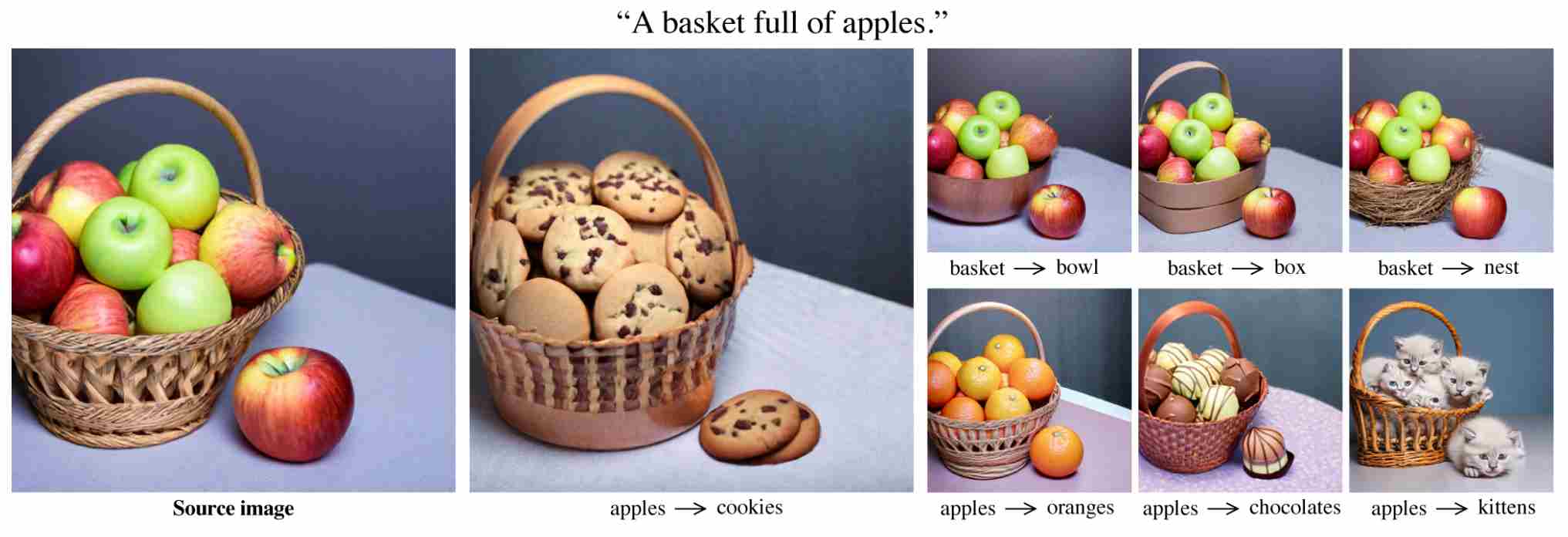
Prompt-to-Prompt (P2P) 6 aims to enable semantic-level editing of generated images by modifying only the textual prompt—such as replacing nouns, adding attributes, or inserting short phrases—while keeping the underlying diffusion model frozen. Its core objective is to ensure that the resulting image faithfully reflects the new prompt (c’) while preserving all visual aspects of the original prompt (c) that remain unchanged. In other words, P2P seeks to achieve prompt-driven local editing: producing the desired modification (e.g., changing “a cat on a sofa” to “a dog on a sofa”) without altering the scene layout, lighting, or other unaffected content, thus realizing controllable and consistent image manipulation purely through cross-attention guidance during inference.
Some classic applications of P2P are as follows:
Word Swap Examples: In this case, we swap tokens of the original prompt with others, e.g., “a basket with apples.” to “a basket with oranges.”.
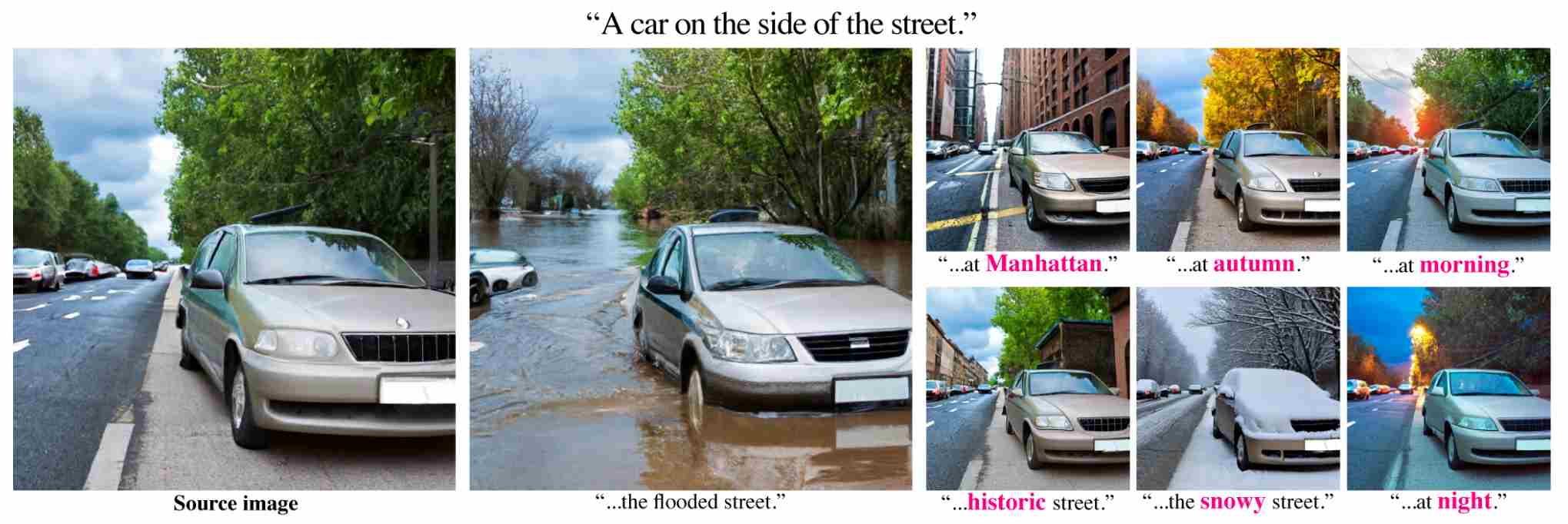
Prompt Refinement Examples: By extending the initial prompt (adding or removing objects) while preserving layout, we perform local or global editing.
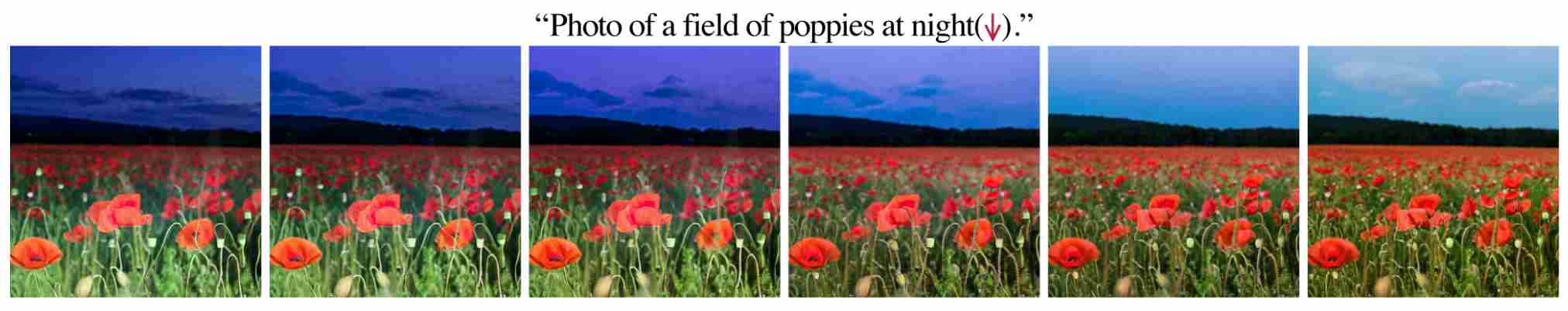
Attention Re-weighting Examples: By reducing or increasing the cross-attention of specific words (marked with an arrow), we control the extent to which it influences the generation.
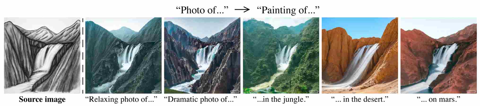
Text-to-Image Style Transfer: By adding a style description to the prompt while injecting the source attention maps, we can create various images in the new desired styles that preserve the structure of the original image.
4.2.1 Core Mechanism: Cross-Attention Replacement/Blending
Classifier-Free Guidance (CFG), which can only enforce global alignment between the text prompt and the generated image, lacking the ability to make fine-grained, localized edits. Similarly, we cannot directly input the modified prompt into the model. This is because even minor changes to the text prompt often result in generated outputs that are drastically different from the original image, thereby violating the principle that some content from the original image must be preserved.
Prompt-to-Prompt overcomes this by intervening directly in the cross-attention maps of the diffusion UNet, where each token’s attention defines where that concept appears. By synchronizing two sampling processes (source and target prompts) and replacing or blending the attention columns of edited tokens (e.g., “cat”→“dog”) while keeping others fixed, it enables localized semantic modifications without retraining or global distortion.
In a cross-attention layer
\[\mathrm{Attn}(Q,K,V)=\mathrm{softmax}\!\left(\frac{QK^\top}{\sqrt{d_k}}\right)V.\]where $Q$ come from image space, whereas $K$ and $V$ come from text token space. The attention map $A=\mathrm{softmax}(QK^\top/\sqrt{d_k})$ determines “where each token looks” — i.e., spatial locations in the image associated with that token.
Element $A_{i,j} \in A$ measures the strength of association between spatial position $i$ and text token $j$. A high value means that the pixel $i$ strongly attends to word $j$.
Column $j$ of $A$ represents the spatial footprint or attention map of the $j^{th}$ text token. It shows where in the image this word exerts influence.
Let $A_s$ denoted as source attention map, $A_t$ denoted as source attention map, the fusion result $\tilde{A}^{(l)}$ is
\[\tilde{A}^{(l)} = M^{(l)} \odot A_t^{(l)} + (1 - M^{(l)}) \odot A_s^{(l)}\]where $M^{(l)}$ is a mask matrix that controls which columns come from the target and which from the source. The modification operations of the attention map vary depending on the differences between the target prompt and the source prompt, with common operations including
| Operation Type | Example (Source → Target) | Attention Map Modification |
|---|---|---|
| Token Replacement | “a dog on the grass” → “a cat on the grass” | $\tilde{A}_{:,col(dog)} = A_t[:,col(cat)]$ Other columns unchanged, copy from $A_s$ |
| Modifier Insertion | “a dog” → “a brown dog” | $\tilde{A} = [A_s[:,a], A_t[:,brown], A_s[:,dog]]$ Re-normalize after insertion |
| Degree Word Insertion | “a cute dog” → “a very cute dog” | $\tilde{A}_{:,cute}=(1+\lambda)A_s[:,cute]$ $\tilde{A}_{:,very}=\eta A_s[:,cute]$ |
| Token Deletion | “a brown dog” → “a dog” | Delete “brown” column: $\tilde{A}=[A_s[:,a],A_s[:,dog]]$ |
| Attribute Strengthening | “a cute dog” → “a very cute dog” or enhance “cute” effect | $\tilde{A}_{:,cute}=(1+\lambda)A_s[:,cute]$ |
| Attribute Weakening | “a very cute dog” → “a cute dog” | $\tilde{A}_{:,cute}=(1-\lambda)A_s[:,cute]$ |
| Token Reordering | “a red big dog” → “a big red dog” | Reorder columns: $\tilde{A}=[A_s[:,a],A_s[:,big],A_s[:,red],A_s[:,dog]]$ |
| Style Injection | “a dog” → “a dog in watercolor style” | High-level blending: $\tilde{A}^{(l)}=(1-\alpha)A_s^{(l)}+\alpha A_t^{(l)}$ ($\alpha≈0.2$) |
4.3 DiffEdit
DiffEdit targets localized, semantically precise edits of a given image using a source prompt $c_s$ that describes the current content and a target prompt $c_t$ that describes the desired change (e.g., “a basket with apples” → “a basket with oranges”). Unlike P2P—which directly manipulates cross-attention—or SDEdit—which relies on global/noisy restarts, DiffEdit automatically discovers where the image should change by contrasting how the denoiser would evolve the same noisy state under (c_s) vs. (c_t). It then performs mask-guided denoising (inpainting) so that only the relevant regions are regenerated while the rest of the image is structurally preserved.
- Inputs: real (or generated) image $x_0$, source prompt $c_s$, target prompt $c_t$, guidance scale (w), diffusion schedule, and an edit noise level $t_{\text{edit}}$ (moderate noise).
- Outputs: edited image $\tilde x_0$ that preserves off-mask content and applies the semantic change inside the discovered mask.
4.3.1 Problem Setting and Intuition
Let $x_0$ be the image to edit. DiffEdit first adds moderate noise to obtain $x_{t_{\text{edit}}}$, then asks: If we start denoising this same state under $c_s$ vs. under $c_t$, where do these two trajectories disagree? Those spatial locations are precisely where the edit should occur. Formally, with a denoiser $\epsilon_\theta$ (CFG form) we compare either the predicted clean image $\hat x_0$ or the predicted noise $\hat\epsilon$ under the two prompts and aggregate deviations across steps into a saliency map that becomes the edit mask.
This yields a two-stage pipeline:
- Mask discovery (where to edit). Contrast $c_s$ vs. $c_t$ on the same noisy states to localize semantic deltas.
- Masked inpainting (how to edit). Run a standard masked sampler that locks off-mask pixels to the original and regenerates only the on-mask region under $c_t$.
4.3.2 Stage I: Automatic Mask Discovery by Trajectory Disagreement
The first step is to discover mask automatically. For this purpose, at a sequence of probe timesteps $t\in\mathcal T\subseteq{t_{\text{edit}},\dots,1}$, we add moderate noise to obtain a sequence of latents $x_t$,for a VP schedule with $\bar\alpha_t$,
\[x_t\;=\;\sqrt{\bar\alpha_{t}}\;x_0 \;+; \sqrt{1-\bar\alpha_{t}}\;\epsilon,\quad \epsilon\sim\mathcal N(0,I).\]execute One-step “probes” under the two prompts ($c_s$ and $c_t$) starting from the same state $x_t$
\[\hat\epsilon_{s}(x_t,t)=\epsilon_\theta(x_t,t\;c_s,\varnothing,w),\qquad \hat\epsilon_{t}(x_t,t)=\epsilon_\theta(x_t,t\;c_t,\varnothing,w).\]Measure token-agnostic semantic deltas with an $L_2$ deviation at each probe step:
\[D^{(t)}_{\epsilon} \;=\; \big\|\hat\epsilon_{t}(x_t,t)-\hat\epsilon_{s}(x_t,t)\big\|_2\label{eq:d_e}\]Accumulate and smooth:
\[D_{\text{agg}}\;=\;\sum_{t\in\mathcal T} D^{(t)}_{\epsilon}\]Then threshold to obtain a soft or hard mask:
\[M \;=\; \mathsf{Normalize}(D_{\text{agg}})>\tau,\]optionally applying morphological open/close to remove speckles and fill small holes. The result \(M\in[0,1]^{H\times W}\) highlights where the model predicts changes under (c_t) vs. (c_s).
We can also measure token-agnostic semantic via $x_0$, prediction, in such case, we replace equation \ref{eq:d_e} with
\[D^{(t)}_{x_0} \;=\; \big\|\hat x_{0,t}^{(t)}-\hat x_{0,s}^{(t)}\big\|_2.\]where
\[\hat x_0^{(t)} \;=\; \frac{x_t-\sqrt{1-\bar\alpha_t}\,\hat\epsilon(\cdot)}{\sqrt{\bar\alpha_t}}.\]4.3.3 Stage II: Mask-Guided Denoising (Inpainting) under the Target Prompt
With $M$ fixed, we now edit only on $M$ while preserving the complement $(1-M)$. Starting again from a noisy state (reuse $t_{\text{edit}}$ or a nearby value), perform a masked reverse process to step down to $t=0$. A practical and stable update (DDIM form, $\eta{=}0$) is:
Compute the standard target-prompt prediction:
\[\hat\epsilon_t\;=\;\epsilon_\theta(x_t,t\;c_t,\varnothing,w)\,\qquad \hat x_0^{(t)}\;=\;\frac{x_t-\sqrt{1-\bar\alpha_t}\,\hat\epsilon_t}{\sqrt{\bar\alpha_t}}.\]Form the masked reconstruction mixing original pixels outside the mask:
\[\hat x_{0,\text{mix}}^{(t)} \;=\; (1-M)\odot x_0 \;+\; M\odot \hat x_0^{(t)}.\]Re-encode to the next latent with the standard DDIM deterministic map:
\[x_{t-1}\;=\;\sqrt{\bar\alpha_{t-1}}\;\hat x_{0,\text{mix}}^{(t)} \;+\; \sqrt{1-\bar\alpha_{t-1}}\;\hat\epsilon_t.\]
This locks off-mask content to the original image at every step, preventing drift, while allowing on-mask regions to follow the target prompt’s generative trajectory. Stochastic SDE variants are analogous, replacing the DDIM step with a masked VP/VE update and noise annealing that matches (\sigma(t)).
4.4 InstructPix2Pix: Instruction-Based Image Editing via Synthetic Supervision
InstructPix2Pix 7 addresses the problem of instruction-based image editing—modifying a given image according to a natural-language command such as “make it look like night,” “add fireworks in the sky,” or “turn this man into a zombie.” Unlike P2P, SDEdit, or DiffEdit, which rely purely on inference-time manipulations, InstructPix2Pix is a retrained diffusion model that learns to execute textual editing instructions directly. Its central idea is simple yet powerful: synthesize large-scale triplets of (input caption, instruction, edited caption) using GPT-3, generate corresponding image pairs with Stable Diffusion, and train a new latent diffusion model that maps
\[(x_\text{before}, \text{instruction}) \;\rightarrow\; x_\text{after}.\]In summary, InstructPix2Pix treats instruction-based image editing as a supervised learning problem. This yields a single model capable of performing arbitrary edits on real images without any inversion, mask, or prompt engineering at inference time.
4.4.1 Motivation and Task Definition
Previous methods such as Prompt-to-Prompt (semantic control), SDEdit (structure-preserving re-denoising), and DiffEdit (mask-based semantic differencing) enable fine-grained edits but still require explicit prompts, mask estimation, or paired generation trajectories.
In contrast, InstructPix2Pix aims to learn a direct mapping between an image and a high-level textual instruction that describes the desired modification. The goal is to model:
\[p_\theta(x_\text{after} \mid x_\text{before}, \text{instruction})\]without any manual intervention or handcrafted editing operations.
4.4.2 Stage I: Synthetic Data Generation
The first step is to construct a large-scale textual editing corpus using a fine-tuned GPT-3 language model. Starting from millions of captions from the LAION-Aesthetics V2 dataset (e.g., “a photo of a girl riding a horse”), GPT-3 generates corresponding instruction–edit pairs:
| Original Caption | Editing Instruction | Edited Caption |
|---|---|---|
| “a girl riding a horse” | “have her ride a dragon” | “a girl riding a dragon” |
| “Yefim Volkov, Misty Morning” | “make it afternoon” | “Yefim Volkov, Misty Afternoon” |
| “Kate Hudson arriving at the Golden Globes” | “make her look like a zombie” | “Zombie Kate Hudson arriving at the Golden Globes” |
Thus each sample forms a triplet: \((\text{caption}*\text{before},; \text{instruction},; \text{caption}*\text{after})\).
This process was repeated across hundreds of thousands of captions, yielding roughly 450 K textual triplets that describe plausible edit operations.
For each triplet, Stable Diffusion (SD) is used to render both before/after images. To ensure the two images differ only in the edited region, Prompt-to-Prompt (P2P) 6 attention control is employed during generation: both prompts share the same random seed and synchronized denoising trajectory, so that layout and structure remain consistent while only the semantically affected region changes.
Each pair is further filtered via CLIP-direction similarity, keeping examples whose textual and visual differences are aligned. The final dataset thus consists of aligned triplets, which is used for supervised diffusion training.
\[(x_\text{before},; \text{instruction},; x_\text{after})\]4.4.3 Stage II: Training the Instruction-Following Diffusion Model
The model is based on Stable Diffusion v1.5, operating in latent space. Given latent $ z_0 = E(x_\text{before}) $ and timestep $ t $, the forward diffusion adds Gaussian noise:
\[z_t = \sqrt{\bar{\alpha}_t}\, z_0 + \sqrt{1-\bar{\alpha}_t}\, \epsilon, \qquad \epsilon \sim \mathcal{N}(0,I).\]The denoiser $ \epsilon_\theta $ predicts noise conditioned on both the image condition and the textual instruction:
\[\epsilon_\theta(z_t, t, E(x_\text{before}), \text{instruction}).\]The training objective is the standard MSE:
\[\mathcal{L} = \mathbb{E}_{z_0,t,\epsilon}\big[\|\epsilon - \epsilon*\theta(z_t, t, E(x_\text{before}), \text{instruction})\|_2^2\big].\]4.4.4 Inference: Dual Classifier-Free Guidance (CFG)
At inference, two CFG scales are applied—one for preserving the input image and another for following the instruction:
\[\begin{align} \tilde{\epsilon}_\theta = & \epsilon_\theta(z_t, \varnothing, \varnothing) + \\[10pt] & s_I\,[\,\epsilon_\theta(z_t, E(x_\text{before}), \varnothing) - \epsilon_\theta(z_t, \varnothing, \varnothing)\,] + \\[10pt] & s_T\,[\,\epsilon_\theta(z_t, E(x_\text{before}), \text{instruction}) - \epsilon_\theta(z_t, E(x_\text{before}), \varnothing)\,] \end{align}\]where $ s_I $ controls structure preservation and $ s_T $ controls editing strength. Typical values are $ s_I \in [1,1.5] $, $ s_T \in [5,10] $. A higher $ s_T $ amplifies instruction compliance, while a higher $ s_I $ enforces stronger resemblance to the original image.
5. Personalized Control: Injecting New Concepts into Diffusion Models
While guidance-based controllable generation (e.g., classifier guidance, ControlNet, or adapter-based conditioning) allows diffusion models to steer the generation process toward a desired attribute, these methods fundamentally operate within the semantic prior already encoded in the pretrained model. In other words, they can emphasize or suppress existing concepts, but cannot truly inject new ones.
However, real-world creative applications—such as personalized avatars, user-specific art styles, product customization, and individualized storytelling—require the model to learn and remember new entities: a particular person, a novel object, a unique texture, or even a newly coined fictional concept that never appeared in the original dataset. This new requirement motivates a distinct research direction: Personalization.
Personalization extends controllable generation from “How to guide the model?” to “How to teach the model something new?” It answers the question of how a diffusion model can absorb new visual or semantic knowledge from a handful of examples, while preserving its generalization ability and aesthetic quality.
5.1 DreamBooth: Model-Side Personalization through Instance-Conditional Fine-Tuning
Pretrained text-to-image diffusion models possess a rich visual prior, capable of synthesizing diverse objects and scenes when guided by text prompts. However, these models lack the ability to represent personalized or rare concepts that do not exist in the training data—such as a specific person, a pet, or a customized object.
DreamBooth 8 addresses this limitation by fine-tuning the diffusion model on a few instance images (typically 3–10) so that a user-defined placeholder token (e.g., “sks”) can faithfully represent that specific subject in generation tasks.
5.1.1 Problem Formulation and Method
Given a pretrained text-to-image diffusion model
\[\epsilon_\theta(z_t, t, \mathcal{T}(c)),\]where $z_t$ is the noisy latent at timestep $t$, $\mathcal{T}(\cdot)$ denotes the text encoder (e.g., CLIP), and $c$ is the text condition, the goal of DreamBooth is to endow the model with a new concept token (e.g., $[\text{sks}]$) that refers to a specific instance (such as “my dog”). To achieve this, DreamBooth constructs two small datasets:
Instance set, containing a few real images of the target subject, with prompts that include both the placeholder token (
\[\mathcal{D}_\text{inst} = {(x_i, c_i)}, \quad c_i = \text{"a photo of sks dog"}\]sks) and its base class word (dog).Class set, consisting of generic examples of the same class, either sampled from the pretrained model or from an external dataset, to maintain category-level generalization.
\[\mathcal{D}_\text{class} = {(\tilde{x}_j, \tilde{c}_j)}, \quad \tilde{c}_j = \text{“a photo of dog”}\]
The dual dataset setup allows the model to learn the new instance without catastrophic forgetting of the base class.
For each training step, images from both datasets are encoded into the latent space via the VAE encoder and corrupted with Gaussian noise:
\[z_0 = \text{Encoder}(x) \quad \Longrightarrow \quad z_t = \sqrt{\bar{\alpha}_t} z_0 + \sqrt{1-\bar{\alpha}_t}\, \epsilon, \quad \epsilon \sim \mathcal{N}(0, I).\]The total loss function combines an instance reconstruction loss and a class prior preservation loss:
\[\mathcal{L}(\theta) = \underbrace{\mathbb{E}_{(x,c)\sim\mathcal{D}_\text{inst}} \!\left[\, \|\epsilon - \epsilon_\theta(z_t, t, \mathcal{T}(c))\|^2 \,\right]}_{\text{instance reconstruction loss}} + \lambda\,\underbrace{\mathbb{E}_{(\tilde{x},\tilde{c})\sim\mathcal{D}_\text{class}} \!\left[\, \|\epsilon - \epsilon_\theta(\tilde{z}_t, t, \mathcal{T}(\tilde{c}))\|^2 \,\right]}_{\text{class prior preservation loss}}\]where $\lambda$ balances instance learning and prior preservation.
- The first term teaches the model that
[sks]corresponds to the specific instance. - The second term constrains the model so that it still generates diverse “dogs” rather than overfitting all dogs to the target one.
5.1.2 Role of the Placeholder Token
The placeholder token [sks] has no prior semantic meaning. By placing it next to its base class (e.g., “dog”) in the text prompt "a photo of sks dog", the model effectively learns a new embedding $e_{\text{sks}}$, such that the combined prompt
where $\delta_{\text{sks}}$ is a semantic offset capturing the idiosyncratic attributes of the target instance—its color, shape, and texture. If “sks” were used alone, the model could not anchor it to the visual distribution of dogs, leading to overfitting or meaningless outputs. Therefore, the co-occurrence of placeholder + class word is crucial for semantic grounding.
In practice, the new token [sks] would be added directly to the tokenizer’s vocabulary and create a new trainable embedding vector $e_{\text{sks}}$, during the training process, the text encoder will be frozen except for the new token embedding. This keeps the language manifold stable while allowing the new token to occupy a precise semantic location relative to its base class.
5.1.3 Best Practices for Parameter Update
DreamBooth fine-tuning updates two parts of the model:
UNet (or DiT) — the generative backbone responsible for denoising.
- In early implementations, the entire UNet was fine-tuned;
- In modern practice, only lightweight LoRA adapters are trained to reduce cost and preserve generality.
Text Encoder — partially updated:
- Only the new token embedding $e_\text{sks}$ is learned or slightly adapted;
- The rest of the text encoder (e.g., CLIP transformer layers) remains frozen to maintain language consistency.
Hence, DreamBooth can be viewed as jointly optimizing the UNet’s visual mapping and the new token’s semantic anchor.
During training process, instance images dataset $(\mathcal{D}_\text{inst})$ are small, typically 3–10 photos. However, several conditions must be met to achieve good results:
- Should cover varied poses, lighting, and backgrounds.
- Background diversity helps prevent overfitting to non-essential details.
- Moderate data augmentation (cropping, jitter, color shift) is encouraged.
Class images dataset $(\mathcal{D}_\text{class})$ are relatively larger, typically 50–500 images of the general class, usually generated by the same pretrained model with prompts like “a photo of dog”.
Typical training batches mix instance and class samples in a 1:1 or 1:2 ratio.
5.2 Textual Inversion: Embedding-Side Personalization via Semantic Optimization
While DreamBooth fine-tunes the generative backbone to represent new concepts, it still requires model adaptation and non-trivial compute. Textual Inversion (TI) 9 offers an extreme parameter-efficient alternative: it keeps the entire diffusion model frozen and learns only one or a few embedding vectors in the text-encoder space that correspond to a new token.
This lightweight method adds a new “word” to the model’s lexicon so that the pretrained generator can synthesize unseen concepts (styles, materials, identities) through language alone.
5.2.1 Problem Formulation and Method
Let the pretrained text-to-image diffusion model be
\[\epsilon_\theta(z_t,t,\mathcal{T}(c)),\]where the parameters $\theta$ of the denoiser (UNet or DiT), the VAE, and the text encoder $\mathcal{T}$ are fixed. We introduce a new token (\tau) (not in the original vocabulary) with trainable embedding $e_\tau\in\mathbb{R}^d$. Given a small set of instance images ${x_i}{i=1}^N$ (typically $N$ is 3–15), Textual Inversion aims to learn $e\tau$ such that prompts containing $\tau$ (e.g., “a photo of \tau dog”) elicit images consistent with those instances, without altering any pretrained weights.
The training data consists solely of the user-provided instance images ${x_i}$. Each image is paired with one or more template prompts to improve generalization:
\[\begin{align} & c_i = \text{“a photo of }\tau\text{ dog”},\\[10pt] & c_i' = \text{“a portrait of }\tau\text{ person”},\\[10pt] & c_i'' = \text{“a painting in the style of }\tau\text{”},;\text{etc.} \end{align}\]The use of multiple syntactic patterns prevents overfitting to a single linguistic context and allows $\tau$ to function as a versatile modifier in novel sentences.
Like DreamBooth, for each image $x$, the VAE encoder produces a latent representation $z_0=\text{Encoder}(x)$. A noise sample $\epsilon\sim\mathcal{N}(0,I)$ and timestep $t$ are drawn to construct the noisy latent:
\[z_t = \sqrt{\bar\alpha_t},z_0 + \sqrt{1-\bar\alpha_t},\epsilon.\]The only trainable variable is $e_\tau$. The objective minimizes the denoising reconstruction loss:
\[\mathcal{L}(e_\tau) =\mathbb{E}_{x,t,\epsilon} \Big[\, \|\epsilon-\epsilon_\theta(z_t,t,\mathcal{T}(c(\tau)))\|_2^2 \,\Big]\]where $c(\tau)$ is the prompt containing the new token. Gradients propagate solely through $e_\tau$; all other parameters remain frozen.
5.2.2 Comparison to DreamBooth
Thus, Textual Inversion can be regarded as a language-space analog of DreamBooth—a purely embedding-level personalization that leverages the pretrained alignment between text and image modalities.
| Aspect | Textual Inversion | DreamBooth |
|---|---|---|
| Updated parameters | Only token embedding ((e_\tau)) | UNet/DiT (+ LoRA) + token embedding |
| Model frozen? | Entirely frozen | Partially trainable |
| Training data | 3–15 images | 3–10 instance + class images |
| Computation cost | Minutes on single GPU | Hours on GPU(s) |
| Expressive power | Good for style/texture | Strong for identity/geometry |
| Portability | Plug-and-play across models | Tied to fine-tuned weights |
6. Structured Condition Control
9. References
Dhariwal P, Nichol A. Diffusion models beat gans on image synthesis[J]. Advances in neural information processing systems, 2021, 34: 8780-8794. ↩
Ho J, Salimans T. Classifier-free diffusion guidance[J]. arXiv preprint arXiv:2207.12598, 2022. ↩
Mokady, Ron, et al. “Null-text inversion for editing real images using guided diffusion models.” Proceedings of the IEEE/CVF conference on computer vision and pattern recognition. 2023. ↩
Miyake D, Iohara A, Saito Y, et al. Negative-prompt inversion: Fast image inversion for editing with text-guided diffusion models[C]//2025 IEEE/CVF Winter Conference on Applications of Computer Vision (WACV). IEEE, 2025: 2063-2072. ↩
Meng, C., et al. “SDEdit: Guided image synthesis and editing with stochastic differential equations.” International Conference on Learning Representations (ICLR), 2022. ↩
Hertz, Amir, et al. “Prompt-to-prompt image editing with cross attention control.” arXiv preprint arXiv:2208.01626 (2022). ↩ ↩2
Brooks T, Holynski A, Efros A A. Instructpix2pix: Learning to follow image editing instructions[C]//Proceedings of the IEEE/CVF conference on computer vision and pattern recognition. 2023: 18392-18402. ↩
Ruiz N, Li Y, Jampani V, et al. Dreambooth: Fine tuning text-to-image diffusion models for subject-driven generation[C]//Proceedings of the IEEE/CVF conference on computer vision and pattern recognition. 2023: 22500-22510. ↩
Gal R, Alaluf Y, Atzmon Y, et al. An image is worth one word: Personalizing text-to-image generation using textual inversion[J]. arXiv preprint arXiv:2208.01618, 2022. ↩