Diffusion models (DMs) and score-based generative models (SGMs) have demonstrated remarkable generative capability, but their iterative sampling procedures require hundreds of function evaluations to approximate the underlying ODE or SDE trajectories accurately. Thus, recent research aims to accelerate generation by distilling multi-step samplers into compact one-step or few-step models.

Consistency Models (CMs) ^{1 2 3} were proposed as a principled framework to enable one-step generation while retaining the expressive power of diffusion processes. The central idea is to directly learn a consistent mapping across the continuous trajectory of the diffusion ODE, such that predictions made at any two time steps $ t $ and $ s $ remain consistent with the same underlying data point $ x_0 $.

Figure 1: Consistency Model

1. Foundation and Preliminaries

To lay the theoretical foundation for subsequent sections, we begin by formalizing the problem setting and the probabilistic dynamics underlying the consistency family. This formulation not only clarifies the relationship between diffusion trajectories and their corresponding probability flow ODEs but also provides a unified lens for understanding both discrete and continuous consistency objectives. The following subsection defines the general setting, the forward perturbation process, and the consistency function, establishing a consistent notation framework used throughout the paper.

1.1 Problem Definition

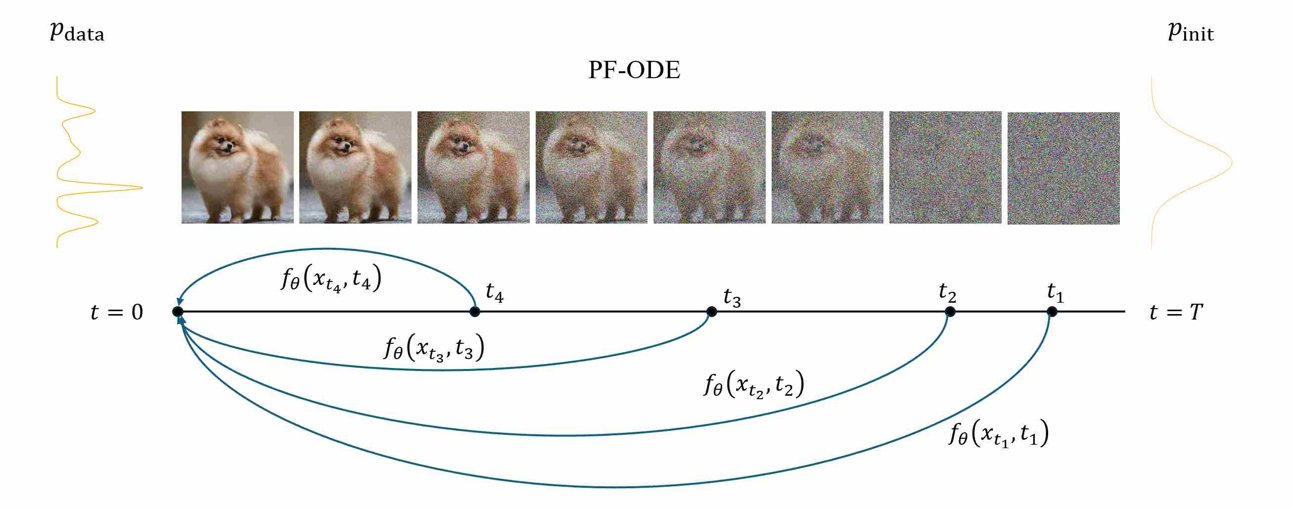
Define the forward Gaussian probability path (forward diffusion process).

Recall that in the first article, we introduced that its corresponding continuous PF-ODE is

This ODE satisfies the continuity equation, ensuring that the trajectory \(\{x_t\}_{t\in [0,1]}\) obtained along this ODE preserves the same time-dependent marginal densities as the stochastic perturbation process.

Let $\Phi_{t\to s}$ denote the exact PF-ODE flow that maps a state at time $t$ to time $s\le t$.

A consistency function \(f_\theta(x_t, t)\) is defined such that it is invariant along the ODE trajectory:

where \(x_s=\Phi_{t\to s}(x_t)\). $f_\theta$ satisfies the boundary condition

This consistency condition implies that $ f_\theta $ remains constant along the trajectory of any valid ODE solution, effectively representing the same clean data point regardless of the diffusion time.

Intuitively, $ f_\theta(x_t, t) $ should project any noisy sample $ x_t $ back to its corresponding clean example $ x_0 $, while maintaining mutual consistency between predictions across all time steps.

1.2 From Definition to Training Paradigms

Although the definition of a consistency function $f_\theta(x_t, t)$ is conceptually elegant—requiring invariance along the diffusion ODE trajectory— it is non-trivial to enforce directly in practice.

In real data, we only observe noisy samples $ x_t $ drawn from the marginal distribution $ p_t(x) $, without access to the exact trajectory or the corresponding clean target $ x_0 $. Therefore, we must design tractable training objectives that approximate this ideal invariance property. Two complementary approaches naturally emerge:

1. Consistency Distillation (CD): If a teacher generative model (e.g., a pretrained diffusion model or an ODE solver) is available, it can serve as a proxy for the true trajectory. The student consistency model learns to reproduce the teacher’s behavior by enforcing that its prediction at time $ t $ remains consistent with the teacher’s prediction at a previous time $ s<t $.

   This yields a teacher-supervised learning paradigm that leverages the high-fidelity trajectory of the pretrained diffusion model.

2. Consistency Training (CT): When no teacher model is available, consistency can still be enforced self-supervisedly. The model ensures that its own predictions at two nearby timesteps are consistent with each other, effectively learning to preserve invariance along the diffusion path.

   This strategy removes external supervision but introduces greater challenges in stability and convergence.

Hence, the two paradigms differ primarily in whether the supervision comes from a teacher model (CD) or from the model’s own temporal consistency (CT). Both share the same theoretical goal: to make $ f_\theta(x_t, t) $ constant along the ODE trajectory, thereby enabling direct one-step generation without explicit integration. The training objective is defined at two adjacent time steps with finite distance:

where $w(t)$ is the weighting function, \(\Delta t > 0\) is the distance between adjacent time steps, and \(d(\cdot, \cdot)\) is a metric function which is used to measure the similarity between two high-dimensional vectors, common choices of $d$ including but not limited to: $L_2$ Loss, Pseudo-Huber Loss, and LPIPS Loss. In our following discussion, we will use $L_2$ Loss for analysis.

2. Teacher-Guided Consistency Distillation

The Consistency Distillation (CD) paradigm assumes the existence of a pretrained teacher model $ g_\phi(x_t, t) $, such as a diffusion model or a deterministic sampler derived from it. The teacher provides a reliable target trajectory for supervision.

Given two time steps $t_n$ and $t_{n-1}=t_n-\Delta t$, the teacher integrates one ODE step to approximate the previous state:

The student consistency model $ f_\theta $ is then trained to match this target:

2.1 Training Pipeline of CD

The consistency-distillation pipeline can be summarized into the following steps:

• Step 1: Sample $x_0$ from the dataset and create a noisy $x_{t_n}$ from forward diffusion process

  \[x_t = s(t)\,x_0 + \sigma(t)\,\epsilon,\qquad \epsilon \in \mathcal N(0,I)\]

• Step 2: Use the pretrained diffusion model $s_{\theta}$ to integrate one ODE step to obtain adjacent position.

  \[\hat{x}_{t_{n-1}} = \Phi_{t_n \to t_{n-1}}(x_{t_n}; g_\phi)\]

  For example, if we have an EDM-Style pre-trained teacher model with $s(t)=1$ and $\sigma(t)=t$, then the PF-ODE is defined by:

  \[dx_t = -t\,s_{\theta}(x_t, t)\,dt\]

  Then, the adjacent position can be approximated by Euler one step.

  \[\hat{x}_{t_{n-1}} \,\approx\, x_{t_{n}} + (t_{n} - t_{n-1})t_n\,s_{\theta}(x_{t_n}, {t_n})\label{eq:next}\]

  We now have a pair sample \((x_{t_n}, \hat{x}_{t_{n-1}})\) that lies on the same path.

• Step 3: Train the objective function (Eq. \ref{eq:cd}) using the collected sample pairs, and solve for the optimal model parameters with optimization algorithms such as gradient descent. In practice, the adjacent point $(x_{t_{n-1}}, t_{n-1})$ is estimated by an EMA network for stability.

  \[\mathcal L_{\text{CD}} = \mathbb{E}_{x_0, t, \epsilon} \Big[w(t) \, \big\| f_\theta(x_t, t) - f_{\theta^-}(\hat{x}_{t_{n-1}}, t_{n-1}) \big\|_2^2\Big]\]

  where $f_\theta$ and $f_{\theta^-}$ are referred to as the student network and the teacher netfork. $ f_{\theta^-} $ is often implemented as an exponential moving average (EMA) of the student network $f_\theta$:

  \[\theta^- \leftarrow \text{stopgrad} (\mu {\theta^-} + (1-\mu){\theta})\]

2.2 Why Use an EMA Teacher

Using an EMA teacher provides two key benefits:

1. Temporal Stability. The EMA weights represent a temporally smoothed version of the student, filtering out high-frequency oscillations and noise introduced by stochastic gradient updates. This produces more coherent and reliable teacher predictions across training iterations, which is crucial for maintaining a stable distillation target.

2. Implicit Self-Distillation. By updating the teacher gradually, the student always learns from a slightly older but more stable version of itself. This creates a form of self-distillation loop that continuously refines the model’s temporal consistency, improving convergence and reducing overfitting to noisy instantaneous updates.

3. Consistency Training From Scratch

While Consistency Distillation (CD) leverages a high-fidelity teacher model to provide supervision, such a teacher may not always be available, especially when one aims to train a generative model from scratch.

To address this, Consistency Training (CT) introduces a self-supervised alternative that enforces the same principle of temporal invariance without external guidance.

3.1 Unbiased Estimation of Score Model

Recall that in consistency distillation, we rely on a pretrained score model $g_{\phi}$ to approximate the ground truth score function. It turns out that we can avoid this pre-trained score model altogether by leveraging the following unbiased estimator. The key idea is that we use the conditional score, rather than the marginal score, as an estimate of the true score.

We do not know the true marginal probability density $p_t(x_t)$, so we cannot obtain the score directly. However, for a given $x_0$, under the general Gaussian perturbation

the conditional probability density $p_t(x_t \mid x_0)$ follows a Gaussian distribution

and the marginal at time $t$ is the mixture (convolution) of that kernel with the data distribution:

Take the derivative of both sides with respect to $x_t$, using Bayes’ rule

Taking the conditional expectation then gives the unbiased score estimator used by CT:

Specifically, we consider EDM-Style diffusion model with $s(t)=1$ and $\sigma(t)=t$ yields

3.2 From CD to CT via Unbiased Substitution

Since we have obtained an unbiased estimate of the score, substituting \ref{eq:ct_unbias2} into Eq. \ref{eq:next} to get the estimate of the next point.

Intuitively, CT approximates $x_{t_{n-1}}=x_{t−∆t}$ in discrete-time CMs by reusing the same data $x_0$ and noise $\epsilon$ when sampling $x_{t_n}$. The objective function now can be rewritten as

3.3 The Equivalence of CD and CT

Let $\Delta t$ represent the maximum value of two adjacent time intervals

Assume that the distance function \(d(\cdot,\cdot)\) and the target network $f_{\theta^-}$ are twice continuously differentiable with bounded second derivatives, the weighting function $w(t)$ is bounded, and that the expected squared norm of the score \(\mathbb{E}\|\nabla \log p_t(x_t)\|_2^2\) is finite. If the pre-trained score model matches the ground-truth score $s_\phi(x,t) = \nabla_x \log p_t(x)$ and the Euler ODE solver is used, then the following holds:

Hence, in the limit $\Delta t \to 0$ and $ N \to \infty $, optimizing the Consistency Distillation loss is equivalent to optimizing the Consistency Training loss.

The proof is established through a first-order Taylor expansion of the target term in the CD loss and the unbiased score identity derived from the Gaussian corruption process.

• Step 1: Taylor expansion of teacher network. For a given sample $x_{t_{n}}$ and timestep $t_{n}$, CD uses the Euler solver to generate the teacher prediction:

  \[\hat{x}_{t_{n-1}} = x_{t_{n}} + (t_{n} - t_{n-1})\,t_n\,s_\theta(x_{t_n},t_n)\]

  Let \(v_{\theta}(x_{t_n},t_n)=-t_n\,s_\theta(x_{t_n},t_n)\), expanding the target network around $(x_{t_{n}}, t_{n})$ by first-order Taylor expansion

  \[\small \begin{align} f_{\theta^-}(\hat{x}_{t_{n-1}}, t_{n-1}) & = f_{\theta^-}(x_{t_{n}}, t_{n}) + \big[ \partial_x f_{\theta^-}(x_{t_{n}}, t_{n})(\hat{x}_{t_{n-1}}-x_{t_n}) + \partial_t f_{\theta^-}(x_{t_{n}}, t_{n})(t_{n-1}-t_n) \big] + O(\Delta t) \\[10pt] & = f_{\theta^-}(x_{t_{n}}, t_{n}) - \Delta t \big[ \partial_x f_{\theta^-}(x_{t_{n}}, t_{n}) v_{\theta}(x_{t_n}, t_n) + \partial_t f_{\theta^-}(x_{t_{n}}, t_{n}) \big] + O(\Delta t) \end{align}\]

  For CT, we substitute the unbiased score identity induced by the Gaussian corruption kernel:

  \[\small \begin{align} & f_{\theta^-}(x_{t_{n}}, t_{n}) - \Delta t \big[ \partial_x f_{\theta^-}(x_{t_{n}}, t_{n}) v_{\theta}(x_{t_n}, t_n) + \partial_t f_{\theta^-}(x_{t_{n}}, t_{n})\big] + O(\Delta t) \\[10pt] = & f_{\theta^-}(x_{t_{n}}, t_{n}) - \Delta t \big[ \partial_x f_{\theta^-}(x_{t_{n}}, t_{n})t_n\,\frac{x_{t_n}-x_0}{t_n^2} + \partial_t f_{\theta^-}(x_{t_{n}}, t_{n})\big] + O(\Delta t) \\[10pt] = & f_{\theta^-}(x_{t_{n}}, t_{n}) + \big[ \partial_x f_{\theta^-}(x_{t_{n}}, t_{n})(- \Delta t)\frac{x_{t_n}-x_0}{t_n} + \partial_t f_{\theta^-}(x_{t_{n}}, t_{n})(- \Delta t)\big] + O(\Delta t) \\[10pt] = & f_{\theta^-}(x_{t_{n}}+(- \Delta t)\frac{x_{t_n}-x_0}{t_n} , t_n + (- \Delta t)) \\[10pt] = & f_{\theta^-}(x_0+t_{n-1}\frac{x_{t_n}-x_0}{t_n} , t_{n-1}) \end{align}\]

  It means that when we use an unbiased estimator to replace the true score, the Taylor expansion of the teacher network around $(t_n, x_{t_n})$ is first-order equivalent.

• Step 2: Taylor expansion of the Loss function. take taylor expansion of the metric $d$ in its second argument

  \[\mathbb E(d(x, y+\Delta)) = \mathbb E(d(x, y)) + \mathbb E(\partial_2 d(x, y)\cdot \Delta) + o(\Delta)\]

  where \(\partial_2\) means the gradient of the function $d$ with respect to its second argument. This equality holds for any metric function. Consider the loss function of CD.

  \[\mathcal L_{\text{CD}} = \mathbb E(d(x, y+\Delta)) = \mathbb E(d(x, y)) + \mathbb E(\partial_2 d(x, y)\cdot \Delta_{\text{CD}}) + o(\Delta)\]

  where

  \[\begin{align} & x = f_{\theta}(x_{t_n}, t_n), \quad y = f_{\theta^-}(x_{t_{n-1}}, t_{n-1}) \\[10pt] & \Delta_{\text{CD}} = (- \Delta t) \big[ \partial_x f_{\theta^-}(x_{t_{n}}, t_{n}) v_{\theta}(x_{t_n}, t_n) + \partial_t f_{\theta^-}(x_{t_{n}}, t_{n})\big] + O(\Delta t) \end{align}\]

  When it comes to the loss function of CT,

  \[\mathcal L_{\text{CT}} = \mathbb E(d(x, y+\Delta)) = \mathbb E(d(x, y)) + \mathbb E(\partial_2 d(x, y)\cdot \Delta_{\text{CT}}) + o(\Delta)\]

  where

  \[\begin{align} & x = f_{\theta}(x_{t_n}, t_n), \quad y = f_{\theta^-}(x_{t_{n-1}}, t_{n-1}) \\[10pt] & \Delta_{\text{CT}} = (- \Delta t) \big[ \partial_x f_{\theta^-}(x_{t_{n}}, t_{n})\frac{x_{t_n}-x_0}{t_n} + \partial_t f_{\theta^-}(x_{t_{n}}, t_{n})\big] + O(\Delta t) \end{align}\]

  The difference between the $\mathcal L_{\text{CT}}$ and $\mathcal L_{\text{CD}}$ lies in $\Delta$, we have already proven in the step 1 that replacing with an unbiased estimator makes this two first-order equivalent, therefore

  \[\mathcal L_{\text{CD}} = \mathcal L_{\text{CT}} + o(\Delta t)\]

4. From Discrete to Continuous Consistency Models

Despite the empirical success of discrete-time consistency models (CMs) in enabling few-step or even one-step sampling, their formulation inherits several intrinsic limitations stemming from the discretization of the underlying probability-flow ODE. These limitations not only restrict theoretical understanding but also hinder scalability and stability when training at high resolutions or with complex noise schedules. The transition to a continuous-time formulation is therefore not merely an aesthetic reformulation but a principled extension that resolves fundamental weaknesses in the discrete regime.

• Discretization Error and Supervision Bias. Discrete CMs rely on numerical solvers to approximate the transition between two adjacent timesteps, typically using Euler or Runge–Kutta integration. The teacher’s prediction at the earlier step, $\hat{x}_{t-\Delta t}$, is thus an approximation rather than an exact ODE state. This introduces a discretization bias into the training target, which propagates through the loss function.

  When the step size $\Delta t$ is large, this bias becomes significant, and the supervision signal deviates from the true PF-ODE trajectory, deteriorating sample quality.

• Sensitivity to Step-Size Scheduling. The discrete formulation requires a predefined set of timesteps ${t_n}_{n=1}^N$ and an associated weighting schedule $w(t_n)$. Both the choice of step size $\Delta t$ and the weighting function strongly affect convergence and visual fidelity, often necessitating extensive empirical tuning. Moreover, using excessively small steps leads to unstable gradients, while large steps amplify bias.

4.1 From Discrete to Continuous Objective

To overcome the aforementioned discretization bias and parameter sensitivity, we reformulate the discrete-time objective into a continuous-time consistency objective ^{1 4}. This transition is grounded in a rigorous limiting process that connects the finite-step consistency loss to its infinitesimal counterpart. Recall the discrete objective defined between two adjacent timesteps:

Here, $\Delta t > 0$ denotes the step size between consecutive timesteps along the probability-flow ODE trajectory. In practice, $x_{t-\Delta t}$ is obtained by numerically integrating the PF-ODE backward by $\Delta t$, introducing a discretization error of order $O(\Delta t^2)$ (Euler).

We expand the teacher’s prediction around the current point $(x_t, t)$ along the PF-ODE direction:

where the total derivative

represents the tangent of $f_{\theta^-}$ along the PF-ODE trajectory. Substitute Eq. \ref{eq:tmp} into the discrete objective gives

Differentiating Eq. \ref{eq:disc} with respect to $\theta$ (noting $\theta^-$ is stop-grad), we obtain

In the infinitesimal limit $\Delta t \to 0$, the discrepancy $\Delta f_t$ vanishes since $f_\theta$ and $f_{\theta^-}$ represent nearly identical predictions at the same point. Retaining only first-order terms yields the continuous-time gradient form:

the continuous-time consistency model loss can be expressed as:

4.2 Geometric Interpretation of the Continuous Consistency Objective

The newly derived continuous-time consistency objective

introduces a fundamental conceptual shift from enforcing finite-step agreement to maintaining infinitesimal temporal invariance along the PF-ODE trajectory.

Minimizing \(\mathcal{L}_{\text{cont}}\) encourages the student prediction \(f_\theta(x_t,t)\) to be orthogonal to this tangent—i.e., to cancel out any residual temporal variation of the teacher.

When $\tfrac{d}{dt}f_{\theta^-}(x_t,t)=0$, the model reaches its ideal stationary state:

which means the model’s output remains constant over time for any point along the ODE trajectory. Combined with the boundary condition $f_\theta(x_0,0)\approx x_0$, this constant becomes precisely the underlying clean data point $x_0$, ensuring perfect temporal consistency:

4.3 Theoretical Advantages Over Discrete Objectives

The continuous objective offers several key advantages compared with the discrete loss $\mathcal{L}_{\text{disc}}$:

• Elimination of Discretization Error.

  The discrete formulation requires evaluating \(f_{\theta^-}(x_{t-\Delta t},t-\Delta t)\) via numerical integration, which inevitably introduces a discretization bias proportional to $O(\Delta t^2)$.

  In contrast, \(\mathcal{L}_{\text{cont}}\) evaluates the tangent term ${df_{\theta^-}}/{dt}$ analytically via Jacobian–vector products (JVPs), avoiding numerical ODE steps entirely. This yields exact supervision at each time $t$, improving both accuracy and training stability.

• Parameter-Free Temporal Scale.

  Discrete-time CMs are sensitive to the choice of $\Delta t$, and therefore require manually designed schedules for fast convergence.

  In contrast, the continuous form removes the need for predefined step sizes $\Delta t$ or scheduling heuristics. Its weighting function $w(t)$ can now be designed as a smooth function (e.g., based on SNR or perceptual importance), decoupled from discrete grid design, thereby enhancing flexibility and scalability.

5. Stabilizing Consistency Training: Practical Recipes

The continuous-time formulation in Section 4 removes the discretization bias in the supervision signal, but naively optimizing the continuous-time objective can still be numerically unstable (and may even underperform discrete-time CMs) unless we carefully control the variance and magnitude of the tangent term. This section summarizes a set of stability-oriented training techniques distilled from the original CM line (CT / CD) and the stabilized continuous-time CM framework (sCM) ^{1 4}.

We focus on techniques that are mechanistically grounded in the continuous-time gradient derived in Section 4, i.e.

where the core difficulty is to estimate and optimize the tangent

5.1 Why Continuous-Time Training Still Becomes Unstable

A useful mental model is: continuous-time CM training is stable iff the tangent is stable. Concretly, the tangent contains two sources of instability:

• Large-magnitude time derivative \(\partial_t f_{\theta^-}\) (or its equivalent inside the chosen parameterization).
• High-variance gradient contributions concentrated at specific time ranges (i.e., poor time-wise conditioning of the objective).

Both issues can occur even when the supervision is “exact” (no discretization bias), because the optimization geometry is still governed by the tangent.

To make the discussion concrete, we follow the TrigFlow-style parameterization adopted by sCM ⁴. Let the forward process be

and define a diffusion backbone $F_\theta$ and the CM predictor

To analyze the stability of tangent function, we first differentiate both sides with respect to $t$:, and then obtain its corresponding expression.

The tangent decomposes into a stable part and a potentially unstable part, the unstable part is typically dominated by the time derivative of the network, which often behaves like

After further analysis, we found instability originates from the time-derivative

where $\mathrm{emb}(\cdot)$ refers to the time embeddings, typically in the form of either positional embeddings or Fourier embeddings. Below we describe improvements to stabilize each component from Eq. \ref{eq:scm}.

5.2 Time Conditioning: Identity Transform and Low-Frequency Embeddings

Technique A: Identity time transform. A simple but crucial choice is

so that

is bounded. This directly prevents the “boundary blow-up” caused by aggressive nonlinear time transforms.

Technique B: Avoid large Fourier scales for $t$-embeddings. For general time embeddings in the form of

we have

With larger Fourier scale $s$, this derivative has greater magnitudes and oscillates more vibrantly, causing worse instability. To avoid this, it is practical to use positional embeddings, which amounts to \(s \approx 0.02\) in Fourier embeddings.

5.3 Conditioning Blocks: Adaptive Double Normalization

The original CM / iCT implementations often use AdaGN-style conditioning inside UNet/DiT blocks.

However, sCM reports that AdaGN can diverge in stabilized continuous-time training, and proposes Adaptive Double Normalization (ADN) as a more numerically robust replacement ⁴.

where pnorm(·) denotes pixel normalization ⁵.

5.4 Objective-Level Stabilization: From Tangent Control to Gradient-Equivalent MSE

This is the core of stabilized training: we do not fight instability by tuning the optimizer, but by controlling the tangent itself and by reparameterizing the objective into a gradient-equivalent squared error.

• Tangent Warmup. Early in training, the estimated tangent is the noisiest. sCM therefore uses a warmup coefficient $r\in[0,1]$ that ramps up the unstable tangent component from 0 to 1 during the first stage of training.

• Tangent Normalization (Clipping in Function Space). Even with warmup, the tangent magnitude can occasionally spike. A direct fix is to normalize the tangent-like target:

  \[g \leftarrow \frac{g}{\|g\| + c},\]

  where $c>0$ prevents division by zero. This is conceptually “gradient clipping”, but applied to the function-space tangent target, which is often more stable than clipping parameter gradients.

• JVP Rearrangement: Make the Tangent Computation Numerically Friendly. Computing $\frac{d}{dt}f_{\theta^-}(x_t,t)$ directly may introduce unnecessary numerical amplification (because $f_{\theta^-}$ itself contains trigonometric factors and nested conditioning). sCM derives an equivalent JVP rearrangement that constructs the training target $g$ from more stable components (notably $F_{\theta^-}$, $\frac{dx_t}{dt}$, and $\frac{d}{dt}F_{\theta^-}$) before applying normalization.

• Gradient-Equivalent “Residual Square” Objective. A subtle but extremely useful trick is: Many CM / diffusion objectives can be written as an inner product between a neural network output and a stop-grad target; the resulting gradient is equivalent to the gradient of a squared error between the network and an “implicit target”.

  Concretely, if we study

  \[\min_\theta\ \mathbb{E}_t\,[F_\theta(t)^\top y(t)]\]

  with stop-grad on $y(t)$, then its gradient is equivalent to

  \[\nabla_\theta\,\mathbb{E}_t\Big[\frac{1}{2}\|F_\theta(t)-F_{\theta^-}(t)+y(t)\|_2^2\Big].\]

  This equivalence is important in practice because it allows you to implement the continuous-time gradient using an MSE-like loss, which is:

  • compatible with standard training code,
  • typically more numerically stable,
  • easier to combine with weighting/normalization tricks.

  This also clarifies why you may see “continuous-time objectives” written in different forms in different papers: they can be gradient-equivalent even if the scalar loss expression looks different.

• Adaptive Weighting Across Time. Even if the tangent is bounded, the loss/gradient variance can still concentrate on a subset of times. sCM adopts an EDM2-style adaptive weighting network $w_\phi(t)$ and optimizes

  \[\min_{\theta,\phi}\ \mathbb{E}_t\left[\frac{e^{w_\phi(t)}}{D}\|F_\theta-F_{\theta^-}+y\|_2^2-w_\phi(t)\right],\]

  which encourages the loss norm to be balanced across times (reducing time-wise variance and improving stability).

6. References