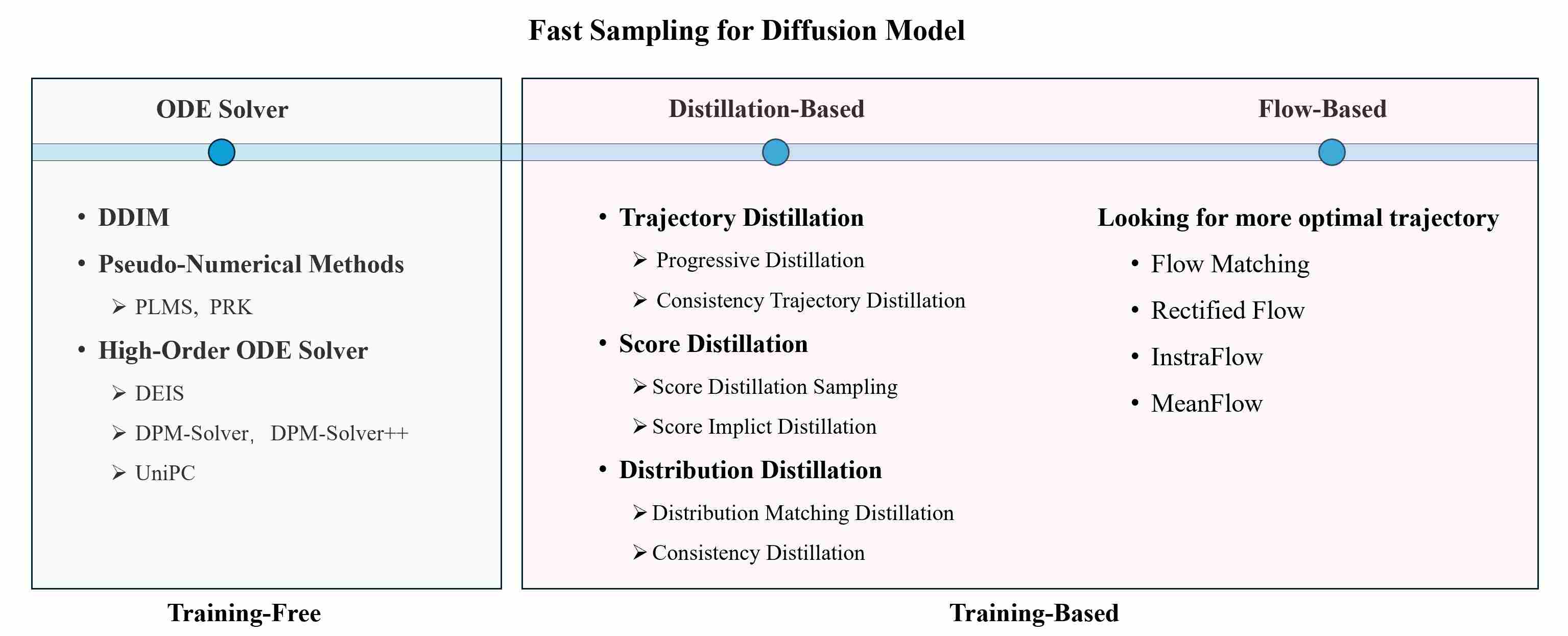
This article systematically reviews the development history of sampling techniques in diffusion models. Starting from the two parallel technical routes of score-based models and DDPM, we explain how they achieve theoretical unification through the SDE/ODE framework. On this basis, we delve into various efficient samplers designed for solving the probability flow ODE (PF-ODE), analyzing the evolutionary motivations from the limitations of classical numerical methods to dedicated solvers such as DPM-Solver. Subsequently, the article shifts its perspective to innovations in the sampling paradigm itself, covering cutting-edge technologies such as consistency models and sampling distillation aimed at achieving single-step/few-step generation. Finally, we combine practical strategies such as hybrid sampling and guidance, conduct a comprehensive comparison of existing methods, and look forward to future research directions such as learnable samplers and hardware-aware optimizations.

1. Introduction

The history of diffusion model sampling is a story of a relentless quest for an ideal balance within a challenging trilemma: Speed vs. Quality vs. Diversity.

• Speed (Computational Cost): The pioneering DDPM (Denoising Diffusion Probabilistic Models) demonstrated remarkable generation quality but required thousands of sequential function evaluations (NFEs) to produce a single sample. This computational burden was a significant barrier to practical, real-time applications and iterative creative workflows. Consequently, the primary driver for a vast body of research has been the aggressive reduction of these sampling steps.

• Quality (Fidelity): A faster sampler is useless if it compromises the model’s generative prowess. The goal is to reduce steps while preserving, or even enhancing, the fidelity of the output. Many methods grapple with issues like error accumulation, which can lead to blurry or artifact-laden results, especially at very low step counts. High-quality sampling means faithfully following the path dictated by the learned model.

• Diversity & Stability: Sampling can be either stochastic (introducing randomness at each step) or deterministic (following a fixed path for a given initial noise). Stochastic samplers can generate a wider variety of outputs from the same starting point, while deterministic ones offer reproducibility. The choice between them is application-dependent, and the stability of the numerical methods used, especially for high-order solvers, is a critical area of research.

This perpetual negotiation between speed, quality, and diversity has fueled a Cambrian explosion of innovative sampling algorithms, each attempting to push the Pareto frontier of what is possible.

2. Classical Generative Models

The essence of any generative model is to build a distribution $p_{\theta}(x)$ to approximate the true data distribution $p_{\text{data}}(x)$, that is,

Once we can evaluate or sample from $p_{\theta}(x)$, we can synthesize new, realistic data.

However, modeling high-dimensional probability densities is notoriously difficult for several intertwined reasons:

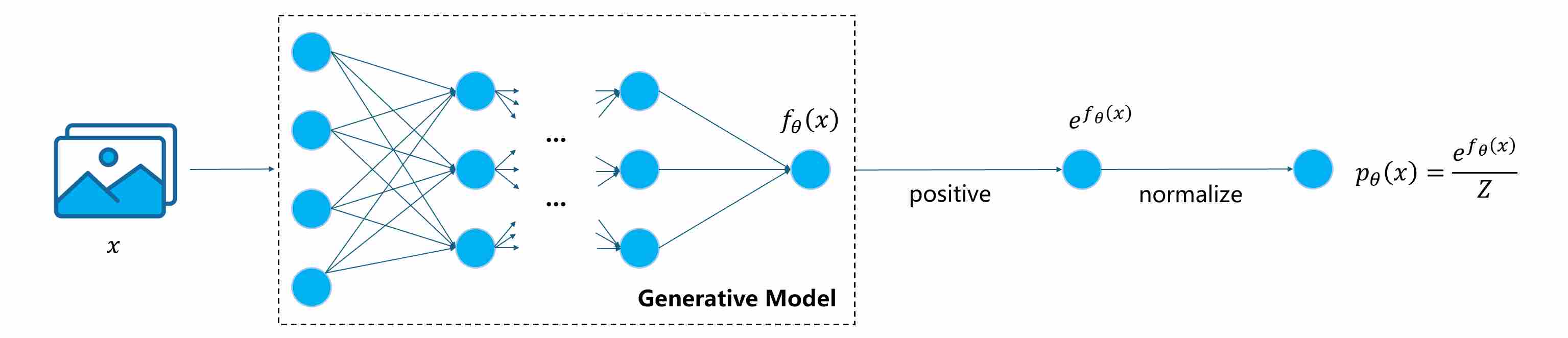
• Intractable Normalization Constant. Many distributions can be expressed as

  \[p_{\theta}(x)=\frac{1}{Z}\,\exp (f_{\theta}(x))\]

  where

  \[Z=\int \exp (f_{\theta}(x))dx\]

  is the partition function. Computing $Z$ in high-dimensional space is intractable, making likelihood evaluation and gradient computation (with respect to $\theta$, not $x$) expensive.

• Curse of Dimensionality. Real-world data (images, audio, text) lies near intricate low-dimensional manifolds within vast ambient spaces. Directly fitting a normalized density over the full space is inefficient and unstable.

• Difficult Likelihood Optimization. To solve $p_{\theta}$, the most common strategy is to optimize $\log p_{\theta}(x)$ (Maximum likelihood estimation). However, maximizing $\log p_{\theta}(x)$ requires differentiating through complex transformations or Jacobian determinants—tractable only for carefully designed, such as flow models.

Although directly estimating the full data density is nearly impossible in high-dimensional space, different classes of generative models have developed specialized mechanisms to avoid or bypass the core obstacles outlined above.

• Variational Autoencoders (VAEs): Approximating the Density via Latent Variables. VAEs sidestep the intractable normalization constant by introducing a latent variable $z$ and decomposing the joint distribution as

  \[p_\theta(x,z)=p_\theta(x \mid z) \cdot p(z),\]

  Instead of maximizing $\log p_\theta(x)$ directly, the VAE introduces an approximate posterior $q_\phi(z\mid x)$ and applies Jensen’s inequality:

  \[\mathcal L_{\text{MLE}} = \log p_\theta(x) \ge \underbrace{ \mathbb E_{q_\phi(z \mid x)}[\log p_\theta(x \mid z)] - \mathrm{KL}(q_\phi(z \mid x) \mid p(z))}_{\mathcal L_{\text{VLB}}}.\]

  Optimizing $\mathcal L_{\text{MLE}}$ requires to compute the gradient of $Z$, which is usually intractable. However, $\mathcal L_{\text{VLB}}$ contains only terms that are individually normalized and easy to compute:

  • $p(z)$ is a simple prior, typically $\mathcal N(0,I)$.

  • $q_\phi(z \mid x)$ is an approximate posterior, which is chosen from a tractable family, e.g.

    \[q_\phi(z\mid x) = \mathcal{N}(z; \mu_\phi(x), \mathrm{diag}(\sigma_\phi^2(x))).\]

    Its log-density is explicitly computable and differentiable with respect to $\phi$.

  • $\log p_\theta(x \mid z)$ is conditional likelihood, which is typically Gaussian or Bernoulli. Since the reconstruction loss is simply the negative log-likelihood of the assumed data distribution given the latent variable. the choice of conditional likelihood determines the form of the reconstructed loss function.

    Conditional Likelihood $p_\theta(x \mid z)$	Reconstruction Loss
    $\mathcal{N}(x; \mu_\theta(z), \sigma^2 I)$	Mean Squared Error (MSE)
    $\mathrm{Bernoulli}(x; \pi_\theta(z))$	Binary Cross Entropy (BCE)
    $\mathrm{Categorical}(x; \pi_\theta(z))$	Cross Entropy
    $\mathrm{Laplace}(x; \mu_\theta(z), b)$	L1 Loss

  Every term in the ELBO depends only on distributions that we define ourselves with explicit normalization constants, this turns an intractable integral into a differentiable objective. Sampling becomes straightforward: draw $z\,\sim\,p(z)$ and decode $x\,\sim\,p_\theta(x \mid z)$. The cost is blurriness in samples—an inevitable consequence of the Gaussian decoder and variational approximation.

• Normalizing Flows: Enforcing Exact Likelihood via Invertible Transformations. Flow-based models make the density tractable by designing the generative process as a sequence of invertible mappings:

  \[x = f_\theta(z),\qquad z\,\sim\,p(z).\]

  The change-of-variables formula yields an explicit, exact log-likelihood:

  \[\log p_\theta(x)=\log p(z)-\log|\det J_{f_\theta}(z)|.\]

  Thus, both density evaluation and sampling are efficient and exact. However, this convenience comes with architectural constraints: each transformation must be bijective with a Jacobian determinant that is computationally cheap to compute. To maintain this property, Flow models (e.g., RealNVP, Glow) restrict the network’s expressiveness compared with unconstrained architectures.

• Generative Adversarial Networks (GANs): Learning without a Normalized Density. GANs abandon likelihoods altogether. A generator $G_\theta(z)$ learns to produce samples whose distribution matches the data via an adversarial discriminator $D_\phi(x)$:

  \[\min_G\max_D ; \mathbb E_{x\sim p_{\text{data}}}\,[\log D(x)] +\mathbb E_{z\sim p(z)}\,[\log(1-D(G(z)))].\]

  This implicit likelihood approach avoids computing $Z$, $\log p(x)$, or any Jacobian. Sampling is trivial: feed a random latent $z$ through the generator. Yet, the absence of an explicit density leads to instability and mode collapse—the model may learn to generate only a subset of modes of the true distribution.

• Energy-Based Models (EBMs): Modeling Unnormalized Densities with MCMC Sampling. EBMs keep the simplest formulation of density—an unnormalized energy function $U_\theta(x)$—but delegate sampling to iterative stochastic processes like Langevin dynamics or Contrastive Divergence. The model defines:

  \[p_\theta(x)=\frac{1}{Z_\theta}\exp(-U_\theta(x)).\]

  Because $Z_\theta$ is intractable, training relies on estimating gradients using samples from the model distribution, obtained via slow MCMC chains. This approach retains full modeling flexibility but sacrifices sampling speed and stability.

3. The Rise of Diffusion Models

Despite their conceptual elegance and individual successes, the classical families of generative models share a common limitation: they struggle to simultaneously ensure expressivity, stability, and tractable likelihoods.

• VAEs approximate densities but pay the price of blurry reconstructions due to their variational relaxation.

• Flow models achieve exact likelihoods, yet the requirement of invertible, volume-preserving mappings imposes severe architectural rigidity.

• GANs generate sharp but unstable samples, suffering from mode collapse and non-convergent adversarial dynamics.

• EBMs enjoy the most general formulation but depend on inefficient MCMC sampling and are notoriously difficult to train at scale.

These obstacles reveal a deeper dilemma: a good generative model must learn both an expressive data distribution and an efficient way to sample from it, but existing paradigms could rarely achieve both at once.

It was precisely this tension—between tractable density estimation and efficient, stable sampling—that motivated the birth of diffusion-based generative modeling. Diffusion models approach generation from an entirely different angle: rather than directly parameterizing a complex distribution, they construct it through a gradual denoising process, transforming simple noise into structured data via a sequence of stochastic or deterministic dynamics. In doing so, diffusion models inherit the statistical soundness of energy-based methods, the stability of likelihood-based training, and the flexibility of implicit generation—thereby overcoming the long-standing trade-offs that constrained previous approaches.

4. The Dual Origins of Diffusion Sampling

Before diffusion models became a unified SDE framework, two independent lines of thought evolved in parallel: One sought to model the gradient of data density in continuous space; the other built an explicit discrete Markov chain that learned to denoise. Both added noise, both removed it—yet for profoundly different reasons.

4.1 The Continuous-State Perspective: Score-Based Generative Models

The first paradigm was rooted in a fundamental question: if we had a function that could always point us toward regions of higher data probability, could we generate data by simply “climbing the probability hill”?

4.1.1 A Radical Shift — Learning the Gradient of data density

Directly modeling $p(x)$ is both theoretically and practically challenging, traditional generative models bypass these challenges through approximation or network structure constraints, but this also limits the model’s performance. One idea is that we do not learn the probability density, but instead learn the gradient of the probability density (also known as score function).

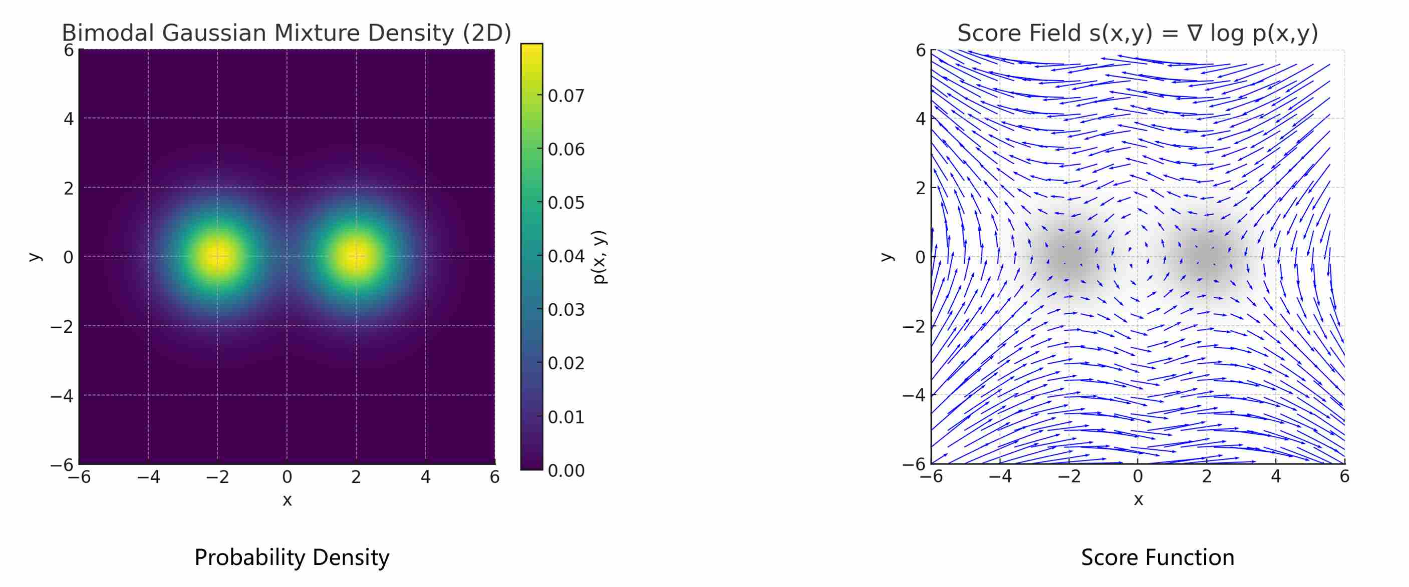
The score function, defined as

As shown in the following figure, score function is a vector field which points toward regions of higher data probability. Learning this vector field—rather than the full density—offers two decisive advantages.

• Independence from the Normalization Constant. Taking the gradient of $\log p(x)$ removes the partition function:

  \[\nabla_x\log p(x) =\nabla_x\log \exp{(f_{\theta}(x))}-\nabla_x\log Z =\nabla_x\log f_{\theta}(x),\]

  because $Z$ is constant w.r.t. $x$. Thus, we can learn meaningful gradients without ever computing $Z$.

• Direction Instead of Magnitude. The score tells us which direction in data space increases probability density the fastest. It defines a probability flow that guides samples toward high-density regions—akin to an energy-based model whose energy is \(U(x)=-\log p(x)\).

• The most important one, is that the probability density and the score provide almost the same useful information, that’s because the score function and the probability density function can be converted between each other: Given the probability density, we can obtain the score by taking the derivative; conversely, given a score, we can recover the probability density by computing integrals.

4.1.2 Score Matching Generative Model

At the heart of this approach lies a powerful mathematical object: the score function, defined as the gradient of the log-probability density of the data, $\nabla_x \log p_{\text{data}}(x)$. Intuitively, the score at any point $x$ is a vector that points in the direction of the steepest ascent in data density. To calculate the score function of any input, we train a neural network $s_{\theta}(x)$ (score model) to learn the score

The loss function is to minimize the Fisher divergence between the true data distribution and the model predicted output:

The challenge, however, is that we do not know the true data distribution $p_{\text{data}}(x)$. This is where Score Matching comes in ¹. Hyvärinen showed that via integration by parts (under suitable boundary conditions), the objective (equation \ref{eq:2}) can be rewritten in a form only involving the model’s parameters:

where $\nabla_x \cdot s_\theta(x) = {\text{trace}(\nabla_x s_\theta(x))}$ is the divergence of the score field. However, SM is not scalable especially for high-dimension data points, because the second term is the jacobin of score model.

For this purpose, Vincent introduced denoising score matching (DSM) ² , by adding Gaussian noise to the real data $x$, the score model becomes predicting the score field of noised data $\tilde{x} = x + \sigma$.

where $p_{\sigma}$ is the data distribution convolved with Gaussian noise of scale $\sigma$, it is easy to verify that predicting $\nabla_{\tilde x} \log p_{\sigma}(\tilde x)$ is equivalent to predict $\nabla_{\tilde{x}} \log p_{\sigma}(\tilde{x} \mid x)$.

When $\sigma$ is small enough, $p_{\text{data}}(x) \approx p_\sigma(\tilde x)$. Optimizing Formula \ref{eq:7} does not require knowing the true data distribution, while also avoiding the computation of the complex Jacobian determinant.

4.1.3 NCSN and Annealed Langevin Dynamics

The first major practical realization of this idea was the Noise-Conditional Score Network (NCSN) ³. However, the authors found that the generated samples by solving \ref{eq:7} with a single small $ \sigma $ are of poor quality, the core issue is that real-world data often lies on a complex, low-dimensional manifold (high-density areas), in the vast empty spaces between data points, the score is ill-defined and difficult to estimate (low-density areas), so low-density regions are underrepresented, leading to poor generalization by the network in those areas. Their solution was ingenious: perturb the data with Gaussian noise of varying magnitudes $\sigma$ ($ \sigma_1 > \sigma_2 > \dots > \sigma_K > 0 $).

• Large $ \sigma_i $: The distribution is highly smoothed, covering the global space with small, stable scores in low-density areas (easier to learn).

• Small $ \sigma_i $: Focuses on local refinement, closer to $ p_{\text{data}} $.

The loss function now can be rewritten as:

With $\lambda{(\sigma)}$ balancing gradients across noise scales and $\mathcal{D}$ is a distribution over $\sigma$. To generate a sample, NCSN employed Annealed Langevin Dynamics (ALD) ³. LD ^{4 5} treats sampling as stochastic gradient ascent on log-density with Gaussian noise injected to guarantees to converge to the target distribution. ALD is an iterative sampling process:

1. Start with a sample drawn from pure noise, corresponding to a very high noise level $\sigma_{\text large}$.

2. Iteratively update the sample using the Langevin dynamics equation:

   \[x_{i+1} \leftarrow x_i + \alpha s_{\theta}(x_i, \sigma_i) + \sqrt{2\alpha}z_i\]

   where $\alpha$ is a step size and $z_i$ is fresh Gaussian noise. This update consists of a “climb” along the score-gradient and a small injection of noise to encourage exploration.

3. Gradually decrease (or “anneal”) the noise level $\sigma_i$ from large to small. This process is analogous to starting with a blurry, high-level structure and progressively refining it with finer details until a clean sample emerges.

4.1.4 Historical Limitations and Enduring Legacy

The NCSN approach was groundbreaking, but it had its limitations. The Langevin sampling process was inherently stochastic due to the injected noise $z$ and slow, requiring many small steps to ensure stability and quality. The annealing schedule itself was often heuristic.

However, its legacy is profound. NCSN established the score function as a fundamental quantity for generative modeling and introduced the critical technique of conditioning on noise levels. It provided the continuous-space intuition that would become indispensable for later theoretical breakthroughs.

4.2 The Discrete-Time Perspective: Denoising Diffusion Probabilistic Models

Running parallel to the score-based work, a second paradigm emerged, built upon the more structured and mathematically elegant framework of Markov chains.

4.2.1 The Core Idea: An Elegant Markov Chain

Independently, Ho et al. ⁶ proposed a probabilistic approach that traded continuous dynamics for a discrete, analytically tractable Markov chain. Instead of estimating scores directly, DDPM proposed a fixed, two-part process.

• Forward (Diffusion) Process: Start with a clean data sample $x_0$. Gradually add a small amount of Gaussian noise at each discrete timestep $t$ over a large number of steps $T$ (typically 1000). This defines a Markov chain $x_0, x_1, \dots, x_T$ where $x_T$ is almost indistinguishable from pure Gaussian noise. This forward process, $q(x_t \mid x_{t-1})$, is fixed and requires no learning.

  \[q(x_t \mid x_{t-1}) = \mathcal{N}(x_t;\,\sqrt{\alpha_t}x_{t-1}, (1-\alpha_t)I)\]

• Reverse (Denoising) Process: Given a noisy sample $x_t$, how do we predict the slightly less noisy $x_{t-1}$? The goal is to learn a reverse model $p_{\theta}(x_{t-1} \mid x_t)$ to inverts this chain.

4.2.2 Forward Diffusion and Reverse Denoising

According to previous post, the solution of DDPM aims to maximize the log-likelihood of $p_{\text data}(x_0)$, which can be reduced to maximizing the variational lower bound, and maximizing the variational lower bound can further be derived as minimizing the KL divergence between $p_{\theta}(x_{t-1} \mid x_t)$ and $q(x_{t-1} \mid x_t, x_0)$.

The true posterior $q(x_{t-1} \mid x_t, x_0)$ can be computed using Bayes’ rule and the Markov property of the forward chain:

Since all three terms in the right sides are Gaussian distribution, the posterior $ q(x_{t-1} \mid x_t, x_0) $ is also Gaussian:

with mean and and variance:

Since our goal is to approximate distribution $ p_{\theta}(x_{t-1} \mid x_t) $ using distribution $q(x_{t-1} \mid x_t, x_0)$, this means that our reverse denoising process must also follow a Gaussian distribution, with the same mean and variance. Because the added noise in the reverse process is unknown, the training objective of DDPM is to predict this noise. We use $\epsilon_{\theta}(x_t, t)$ to represent the predicted noise output, substituting $ \epsilon $ with the noise predicted $\epsilon_{\theta}(x_t, t)$:

where:

Sampling is the direct inverse of the forward process. One starts with pure noise $x_T \sim \mathcal{N}(0, I)$ and iteratively applies the learned reverse step for $ t = T, T-1, \dots, 1$, using the noise prediction $\epsilon_{\theta}(x_t, t)$ at each step to denoise the sample until a clean $x_0$ is obtained.

4.2.3 Theoretical Elegance and Practical Bottleneck

DDPMs offered a strong theoretical foundation, stable training, and state-of-the-art sample quality. However, this came at a steep price: the curse of a thousand steps. The model’s theoretical underpinnings relied on the Markovian assumption and small step sizes, forcing the sampling process to be painstakingly slow and computationally expensive.

4.3 The Initial Convergence: Tying the Two Worlds Together

For a time, these two paradigms—one estimating a continuous gradient field, the other reversing a discrete noise schedule—seemed distinct. Yet, a profound and simple connection lay just beneath the surface. It was shown that the two seemingly different objectives were, in fact, two sides of the same coin.

The score function $s(x_t, t)$ at a given noise level is directly proportional to the optimal noise prediction $\epsilon(x_t, t)$:

where $\sigma_t$ is the standard deviation of the noise at time $t$.

This equivalence is beautiful. Predicting the noise is mathematically equivalent to estimating the score. The score-based view provides the physical intuition of climbing a probability landscape, while the DDPM view provides a stable training objective and a concrete, discrete-time mechanism.

With this link established, the two parallel streams began to merge into a single, powerful river. This convergence set the stage for the next major leap: breaking free from the rigid, one-step-at-a-time sampling of DDPM, and ultimately, the development of a unified SDE/ODE theory that could explain and improve upon both.

5. The First Leap in Efficiency: Breaking the Markovian Chain with DDIM

The stunning quality of DDPMs came at a steep price: the rigid, step-by-step Markovian chain. This constraint, while theoretically elegant, was a practical nightmare, demanding a thousand or more sequential model evaluations for a single image. The field desperately needed a way to accelerate this process without a catastrophic loss in quality. The answer came in the form of Denoising Diffusion Implicit Models (DDIM) ⁷, a clever reformulation that fundamentally altered the generation process.

5.1 From Stochastic Denoising to Deterministic Prediction

The core limitation of the DDPM sampler lies in its definition of the reverse process, which models $p_{\theta}(x_{t-1} \mid x_t)$. This conditional probability is what creates the strict, one-step-at-a-time dependency.

The DDIM paper posed a brilliant question: what if we don’t try to predict $x_{t-1}$ directly? What if, instead, we use our noise-prediction network $\epsilon_{\theta}(x_t, t)$ to make a direct guess at the final, clean image $x_0$? This is surprisingly straightforward. Given $x_t$ and the predicted noise $\epsilon_{\theta}(x_t, t)$, we can rearrange the forward process formula to solve for an estimated $x_0$, which we’ll call $\hat{x}_0$:

This single equation is the conceptual heart of DDIM. By first estimating the final destination $x_0$, we are no longer bound by the previous step. We have a “map” that points from our current noisy location $x_t$ directly to the origin of the trajectory. This frees us from the Markovian assumption and opens the door to a much more flexible generation process.

5.2 The Freedom to Jump: Non-Markovian Skip-Step Sampling

With an estimate of pred \(\hat{x}_0\) in hand, DDIM constructs the next sample $x_{t-1}$ in a completely different way. It essentially says: “Let’s construct $x_{t-1}$ as a weighted average of three components”:

• The “Clean Image” Component: The estimated final image predicted $\hat x_0$, pointing towards the data manifold.

• The “Noise Direction” Component: The direction pointing from the clean image $x_0$ back to the current noisy sample $x_t$, represented by $\epsilon_{\theta}(x_t, t)$.

• A Controllable Noise Component: An optional injection of fresh random noise.

The DDIM update equation is as follows:

Here, \(z_t\) is random noise, and $\sigma_t$ is a new hyperparameter that controls the amount of stochasticity. $\sigma_t = \eta \tilde{\beta}_t$, where $\tilde{\beta}_t$ is defined in DDPM (Equation \ref{eq:14})

This formulation \ref{eq:20} is non-Markovian because the calculation of $x_{t-1}$ explicitly depends on predicted $x_0$, which is an estimate of the trajectory’s origin, not just the immediately preceding state $x_t$. Because this process is no longer Markovian, the “previous” step doesn’t have to be $t-1$. We can choose an arbitrary subsequence of timesteps from the original $1, \dots, T$, for example, $1000, 980, 960, …, 20, 0$. Instead of taking 1000 small steps, we can now take 50 large jumps. At each jump from $t$ to a much earlier $s < t$, the model predicts $x_0$ and then uses the DDIM update rule to deterministically interpolate the correct point $x_s$ on the trajectory. This “skip-step” capability was a game-changer. It allowed users to drastically reduce the number of function evaluations (NFEs) from 1000 down to 50, 20, or even fewer, providing a massive speedup with only a minor degradation in image quality.

Formula \ref{eq:20} also reveals an important theory: for any $x_{t-1}$, the marginal probability density obtained through DDIM sampling is consistent with the marginal probability density of DDPM.

This is why DDIM can take large jumps and still produce high-quality images using a model trained for the one-step DDPM process.

5.3 The $\eta$ Parameter: A Dial for Randomness

DDIM introduced another powerful feature: a parameter denoted as $\eta$ that explicitly controls the stochasticity of the sampling process.

• $\eta = 0$: (Deterministic DDIM): When $\eta = 0$, the random noise term in the update rule is eliminated. For a given initial noise $x_T$, the sampling process will always produce the exact same final image x_0. This is the “implicit” in DDIM’s name, as it defines a deterministic generative process. This property is incredibly useful for tasks that require reproducibility or image manipulation (like SDEdit), as the generation path is fixed.

• $\eta = 1$ (Stochastic DDIM): When $\eta = 1$, DDIM adds a specific amount of stochastic noise at each step. It was shown that this choice makes the marginal distributions $p(x_t)$ match those of the original DDPM sampler. It behaves much like DDPM, offering greater sample diversity at the cost of reproducibility.

• $0 < \eta < 1$ (Hybrid Sampling): Values between 0 and 1 provide a smooth interpolation between a purely deterministic path and a fully stochastic one, giving practitioners a convenient “dial” to trade off between diversity and consistency.

5.4 Bridging to a Deeper Theory: The Lingering Question

DDIM was a massive practical leap forward. It provided the speed that was desperately needed and introduced the fascinating concept of a deterministic generative path. However, its derivation, while mathematically sound, was rooted in the discrete-time formulation of DDPM. The deterministic path ($\eta=0$) worked exceptionally well, but it raised a profound theoretical question:

What is this deterministic path? If a continuous process underlies generation, can we describe this path more fundamentally?

The success of deterministic DDIM strongly hinted that the stochasticity of Langevin Dynamics and DDPM sampling might not be strictly necessary. It suggested the existence of a more fundamental, deterministic flow from noise to data. Explaining the origin and nature of this flow was the next great challenge.

This question sets the stage for our next chapter, where we will discover the grand, unifying framework of Stochastic and Ordinary Differential Equations (SDEs/ODEs), which not only provides the definitive answer but also reveals that Score-Based Models and DDPMs were two sides of the same mathematical coin all along.

6. The Unifying Framework of SDEs and ODEs

The insight behind DDIM—that sampling can follow a deterministic path derived from a learned vector field—opens the door to a more general formulation: diffusion models can be expressed as continuous-time stochastic or deterministic processes. In this chapter, we formalize that insight by introducing the Stochastic Differential Equation (SDE) and the equivalent Probability Flow Ordinary Differential Equation (ODE) perspectives. This unified view provides the theoretical bedrock for nearly all subsequent developments in diffusion sampling, including adaptive solvers, distillation, and consistency models.

6.1 From Discrete Steps to Continuous Time

The core insight is to re-imagine the diffusion process not as $T$ discrete steps, but as a continuous process evolving over a time interval, say $t \in [0, T]$. In this view, $x_0$ is the clean data at $t=0$, and $x_T$ is pure noise at $t=T$. The forward process is no longer a chain but a trajectory governed by a Stochastic Differential Equation (SDE) that continuously injects noise.

Where $f(x_t, t)$ is a drift term, which describes the deterministic part of the SDE’s evolution. $g(t)$ is a diffusion coefficient, which scales the magnitude of the random noise. $dw_t$ is a standard Wiener process, $dw_t=\sqrt{dt}\epsilon,\,\epsilon \sim \mathcal{N}(0, I)$.

This continuous formulation is incredibly powerful because it allows us to leverage the mature and rigorous mathematics of stochastic calculus. More importantly, it was proven by Song et al. in their seminal work that there exists a corresponding reverse-time SDE that can transform pure noise at $t=T$ back into data at $t=0$. This reverse SDE is the true, continuous-time “master equation” for generation.

Where $s_{\theta}(x_t, t)$ is the score function, learned by the neural network. $d{\bar w}_t$ An infinitesimal “kick” from a standard Wiener process (random noise).

This single equation serves as the grand unifier for the stochastic samplers from section 2. Both Annealed Langevin Dynamics (from NCSN) and the DDPM sampling procedure can be shown to be different numerical discretization schemes for this exact same SDE. They were, all along, just two different ways to approximate the solution to one underlying continuous process.

6.2 The Probability Flow ODE: Discovering the Deterministic Path

The reverse SDE provides a complete picture for stochastic generation, but what about the deterministic path discovered by DDIM? This is where the second part of the unified theory comes into play.

For any given SDE that describes the evolution of individual random trajectories, there exists a corresponding Ordinary Differential Equation (ODE) that describes the evolution of the probability density of those trajectories. This is known as the Probability Flow (PF) ODE. While the SDE traces a jagged, random path, the PF-ODE traces a smooth, deterministic “flow” of probability from the noise distribution to the data distribution.

The PF-ODE corresponding to the reverse SDE is:

Notice the two critical differences from the SDE:

1. The diffusion term is gone. There is no more stochastic noise injection. The process is entirely deterministic.
2. The score term $s_{\theta}$ is scaled by $\frac{1}{2}$. This factor arises directly from the mathematical conversion (via the Fokker-Planck equation) from the SDE to its deterministic counterpart.

This ODE is the definitive answer to the puzzle of DDIM. The deterministic path ($\eta = 0$) that DDIM so effectively approximates is, in fact, a trajectory of this very Probability Flow ODE. The DDIM update rule is a specific (and quite effective) numerical solver for this equation.

6.3 A New Paradigm for Sampling

The SDE/ODE framework marks a moment of theoretical completion and a paradigm shift. We now have a single, coherent view that elegantly encompasses all previous methods:

This new perspective immediately begs the next question. The world of numerical analysis has spent over a century developing sophisticated methods for solving ODEs—from simple Euler methods to high-order Runge-Kutta schemes. Can we simply apply these off-the-shelf, classical solvers to the PF-ODE and achieve even greater speed and accuracy?

As we will see in the next chapter, the answer is surprisingly complex. The unique properties of the diffusion PF-ODE present significant challenges to standard numerical methods, necessitating the development of a new class of specialized, “diffusion-aware” solvers.

7. Solver Engineering: High-Order PF-ODE Solver in Diffusion Models

The transition from stochastic sampling (via SDEs) to deterministic sampling (via the Probability Flow ODE) transformed diffusion generation into a numerical integration problem. Once the evolution of data can be written as an ODE,

the task of generating a sample becomes equivalent to integrating this equation backward in time, from random noise at $t = T$ to the data manifold at $t = 0$.

At first glance, this seems to open the door to the rich ecosystem of traditional numerical solvers, such as Euler, Heun, Runge–Kutta, Adams–Bashforth, and so on. However, diffusion sampling presents unique challenges that make these classical algorithms inadequate without adaptation.

7.1 Why Classical ODE Solvers Fall Short

The PF-ODE is not a conventional physics or engineering system but a learned dynamical system defined by a neural network. Classical solvers assume smooth, analytic derivatives and prioritize path fidelity—ensuring each intermediate step closely matches the true trajectory. Diffusion sampling, by contrast, only requires endpoint fidelity: as long as the final state $x_0$ lies on the data manifold, large intermediate deviations are acceptable.

Moreover, evaluating the derivative $\mathbf{f}(t,\mathbf{x})$ involves a full forward pass of a deep neural network (often a U-Net), making every function evaluation costly. High-order solvers that need multiple evaluations per step rapidly become inefficient.

Compounding this, diffusion dynamics are stiff—different dimensions evolve at dramatically different rates—and the learned score field $s_\theta$ is only an approximation, introducing noise and bias that can destabilize high-order methods. These characteristics make standard numerical integration theory ill-suited to the diffusion context.

7.2 The Rise of Specialized Solvers

These difficulties led to a new family of diffusion-aware numerical solvers, designed specifically to balance accuracy, stability, and computational budget. Instead of preserving local precision at every point, these methods explicitly optimize for global fidelity of the terminal sample under limited NFEs (number of function evaluations).

This insight underpins the design of solvers such as DPM-Solver, DPM-Solver++, DEIS, UniPC, and many others, which adapt principles from exponential integrators, predictor–corrector frameworks, and adaptive step-size control to the peculiarities of PF-ODE dynamics. Collectively, they represent a crucial bridge between differential-equation theory and practical, efficient diffusion sampling.

7.3 Beyond This Overview

Because this topic encompasses substantial theoretical and algorithmic depth—including solver derivations, stability analyses, and empirical comparisons—it is discussed separately in a dedicated article. For the complete treatment of high-order PF-ODE solvers, please refer to this post.

8. Consistency Models

High-order PF-ODE solvers (Sec. 7) can reach good quality in 10–20 NFEs, but pushing to few-step (≤4) or single-step generation exposes a fundamental limitation: numerical integration errors dominate when the step size is very large. Instead of integrating along the path, Consistency Models (CMs) learn a function that jumps directly to the endpoint on the data manifold while remaining self-consistent across noise levels.

Concretely, for any intermediate time/noise level $t$ (or $\sigma$), the model should output the same clean sample one would obtain by exactly solving the PF-ODE from that state to $t=0$. This reframes sampling as learning an invariant endpoint map, enabling 1–4 NFE generation with competitive fidelity.

8.1 Principle: consistency as an invariance constraint

Let $\Phi_{t\to s}$ denote the exact PF-ODE flow that maps a state at time $t$ to time $s\le t$.

The endpoint map is $\Phi_{t\to 0}(\,\cdot\,)$. Consistency demands that flowing to any intermediate $s$ and then to $0$ equals flowing directly to $0$:

A consistency function $f_\theta(x_t, t)$ is trained to approximate this endpoint map:

and should satisfy the consistency identity, as shown in the following figure.

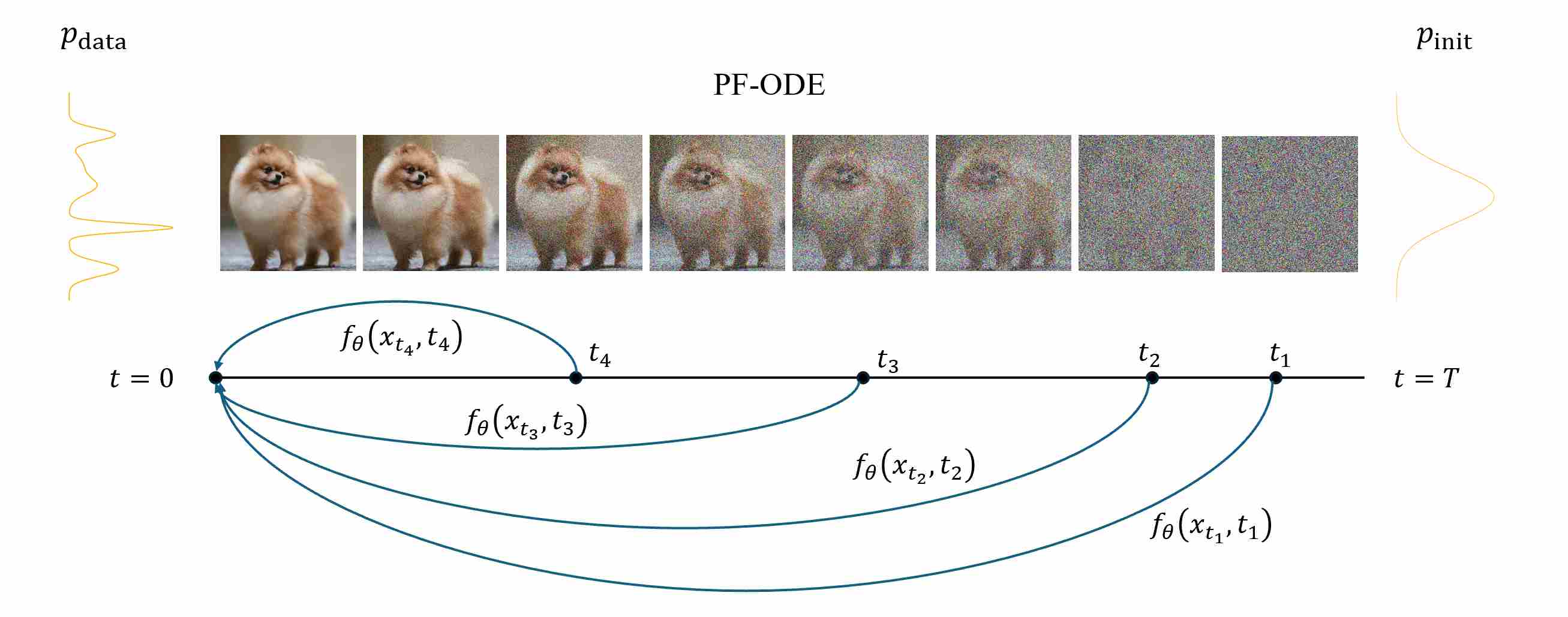
our objective is to minimize the consistency loss between different noise levels,

where $d$ is a distance metric, such as L2 norm, L1 norm, or LPIPS. However, the model could trivially drive the loss to zero by outputting a constant image for all inputs and time steps,

since both sides of the loss would be identical. Such a degenerate solution makes the model independent of the input and destroys its generative ability. In practice, We also add an endpoint boundary constraint:

where $\epsilon$ is a time step that approachs to 0. This boundary constraint plays a crucial role in preventing the collapse problem during training. we anchor the model’s behavior at the noise-free endpoint: it must reproduce the original clean image when $t{=}0$. This boundary condition breaks the trivial constant solution, forcing the network to learn a non-trivial mapping that depends on both the noisy input $x_t$ and the noise level $t$. Intuitively, the constraint defines a fixed point on the data manifold that every predicted trajectory must converge to, ensuring that the model remains meaningful and that its outputs at all noise levels are self-consistency while still faithful to the data distribution.

The core issue of CM lies in how to find $x_{t_{n-1}}$ when given $x_{t_n}$, since $x_{t_n}$ and $x_{t_{n-1}}$ are on the same ODE trajectory, theoretically, given $x_t$, $x_s$ can be obtained by solving the ODE

Here, we use EDM-Style ODE form: \(f(t)=0, g(t)=\sqrt{2t}\). Depending on the different ways of solving the integrals, there can be two different training methods: consistency distillation and consistency training.

8.2 consistency distillation

Consistency Distillation is a method for utilizing a pre-trained diffusion model to obtain an accurate estimate of $x_{t_{n-1}}$ from $x_{t_n}$, by running one discretization step of a numerical ODE solver, $x_{t_{n-1}}$ can be derived from

$s_{\theta}$ is our pre-trained teacher model. The consistency-distillation pipeline can be summarized into the following steps:

• Step 1: Sample $x_0$ from the dataset and create a noisy $x_{t_n} = x_0 + t_n\epsilon$.

• Step 2: Use the pretrained diffusion model $s_{\theta}$ to integrate one ODE step:

  \[x_{t_{n-1}} = x_{t_{n}} - (t_{n-1} - t_{n})t_n s_{\theta}(x_{t_n}, {t_n})\label{eq:cd}\]

  We now have a pair $x_{t_n}, x_{t_{n-1}}$ that lies on the same path.

• Step 3: Define the consistency function $f_{\theta}$ which is trained to produce consistent outputs for this pair. The loss function minimizes the distance between their predictions:

  \[\mathcal L_{\text{CD}} = \mathbb E[d(f_{\theta}(x_{t_n}, t_n), f_{\theta^-}(x_{t_{n-1}}, t_{n-1}))]\]

  where

  \[f_{\theta}(x_t, t) = c_{\text{skip}}x_t + c_{\text{out}}F_{\theta}(c_{\text{in}}x_t, c_{\text{noise}})\]

  and $f_{\theta^-}$ is a target network, typically an exponential moving average (EMA) of $f_{\theta}$’s weights, which provides a more stable training target.

  \[f_{\theta^-} \leftarrow \text{stopgrad} (\mu {\theta^-} + (1-\mu){\theta})\]

  $\theta$ is the network being optimized, ${\theta^-}$ provides a smooth, stop-gradient target.

8.3 consistency training

Consistency models can be trained without relying on any pre-trained diffusion models. Recall equation \ref{eq:cd}, we rely on a pretrained score model $s_{\theta}$ to approximate the ground truth score function $\nabla_{x_t} \log p_t(x_t)$. It turns out that we can avoid this pre-trained score model altogether by leveraging the following unbiased estimator

This unbiased estimate suffices to replace the pre-trained diffusion model in consistency distillation when using the Euler method as the ODE solve. Now, we using equation \ref{eq:ct} and substitute into equation \label{eq:cd}, and get the estimate:

where $x \in p_{\text{data}}$, and $\epsilon \in \mathcal N(0,I)$.

8.4 Consistency Trajectory Model (CTM)

Although Consistency Models (CM) enable single-step or few-step deterministic sampling by directly learning a mapping from any noisy intermediate sample $x_t$ to the clean data $x_0$, their efficiency comes with notable trade-offs.

• First, multi-step generation deteriorates rather than improves image quality—an effect explained by the overlapping time intervals between stochastic jumps.

• Second, CMs lack an explicit score function, preventing likelihood computation and the reuse of controllable generation methods inherited from diffusion models.

• Third, the loss in CM enforces local consistency only toward the zero-time endpoint, ignoring global temporal relations along the ODE trajectory.

To address these limitations, Consistency Trajectory Model (CTM) ⁸ generalizes CM into a unified framework that simultaneously learns the integral form (long-range jumps) and the infinitesimal derivative (local score) of the probability-flow ODE. By introducing a trajectory-consistent neural jump operator $G_\theta(x_t,t,s)$, CTM unifies numerical solvers and distillation approaches within a single network. As a result, CTM maintains consistent generation quality across different NFEs, provides access to an explicit score function, and allows both teacher-guided and teacher-free training.

9. Distillation for fast sampling

Although higher-order ODE solvers (e.g., DPM-Solver++, UniPC) can reduce the number of denoising steps from hundreds to fewer than twenty, the computational cost remains substantial for high-resolution image synthesis and real-time applications. The ultimate goal of sampling acceleration is to achieve few-step or even single-step generation without sacrificing fidelity or diversity.

Distillation-based approaches address this challenge by compressing the multi-step diffusion process into a student model that can approximate the teacher’s distribution within only one or a few evaluations. Unlike numerical solvers, distillation learns a direct functional mapping from noise to data, thereby converting iterative denoising into an amortized process.

9.1 Progressive Distillation

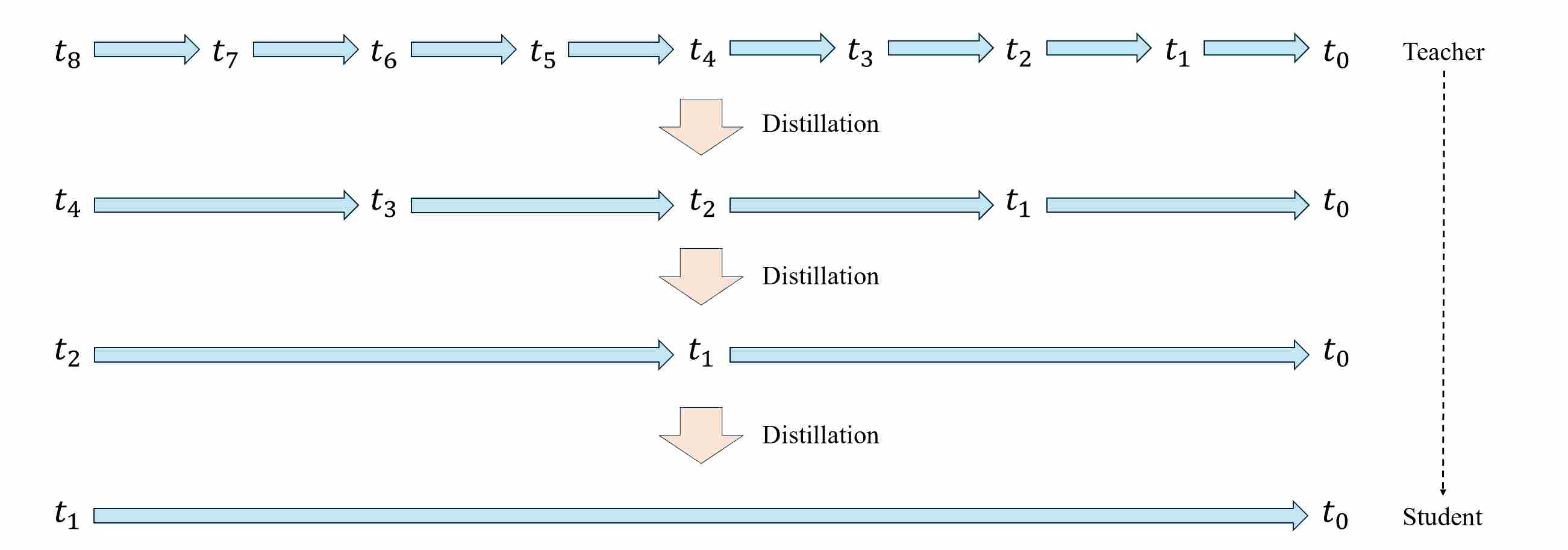
Progressive Distillation (PD) ⁹ compresses a pretrained “teacher” diffusion sampler that runs in $T$ steps into a “student” sampler that runs in $T/2$ steps, then recursively repeats the procedure \((T/2 \rightarrow T/4 \rightarrow \dots)\), typically reaching 4–8 steps with minimal quality loss.

Let \(\{t_n\}_{n=0}^{N}\) be a decreasing time/$\sigma$ grid with $t_0=0$ and $t_N=T$. Denote the teacher’s one-step transition (DDIM/ODE or DDPM/SDE) by

where $\Phi_\theta$ is an ODE Solver. Its two-step composite

A student $f$ with parameters $\phi$ is trained to replace two teacher steps with one:

A visualization of progressive distillation algorithm is shown as follows.

9.1.1 Target Construction and Loss Design

Training pairs are self-supervised by the teacher: Sample $x_{t_n}$ either from $\mathcal N(0,I)$ or by forward noising data \(x_0\sim p_{\text{data}}\) through \(q(x_{t_n} \mid x_0)\). Then, run two teacher steps to get the target state

PD can utilize different targets that we expect the student model to predict in one step from $x_t$, each corresponding to a distinct loss function. $x_{t_{n-2}}^{\text{T}$ is a simple and straightforward target that we expect the student model to predict, with this as the goal, we introduce the PD regression loss.

9.1.2 Strengths and Limitations

Progressive Distillation offers an elegant and empirically robust pathway toward accelerating diffusion sampling. Its main strengths lie in its stability, modularity, and data efficiency.

• Data-free (or data-light): supervision comes from the teacher sampler itself.
• Stable and modular: each stage is a local two-step merge problem.
• Excellent trade-off at 4–8 steps: large speedups with negligible FID/IS degradation.
• Architecture-agnostic: applies to UNet/DiT backbones and both pixel/latent spaces.

However, PD also faces fundamental limitations.

• Produce blurry and over-smoothed output: The MSE loss minimizes the squared difference between the prediction and the target, which mathematically drives the optimal solution toward the conditional mean of all possible teacher outputs.

• One-step limit is hard: local two-step regression accumulates errors when composed; texture/high-freq details degrade.
• Teacher-binding: student quality inherits teacher biases (guidance scale, scheduler, failure modes).
• Compute overhead: multiple PD stages plus teacher inference can approach original pretraining cost (though still typically cheaper).

9.2 Adversarial Diffusion Distillation

While Progressive Distillation (Sec. 9.1) compresses multi-step sampling through supervised teacher-student regression, it still depends on explicit trajectory matching: the student must imitate the teacher’s denoising transitions.

Adversarial Diffusion Distillation (ADD) ¹⁰ proposes a fundamentally different perspective: rather than minimizing a reconstruction distance between teacher and student trajectories, the student is trained adversarially to generate outputs that are indistinguishable from real data, while remaining consistent with the diffusion process implied by the teacher.

9.2.1 Motivation: From Trajectory Matching to Distribution Matching

Distillation frameworks such as PD and CM/CTM explicitly approximate the trajectory of the teacher diffusion ODE—mapping a noisy input $x_t$ to its denoised counterpart $x_{t-\Delta t}$ or directly to $x_0$.

Yet, these approaches inherently assume that the teacher’s trajectory is optimal in both perceptual and statistical senses. In practice, teacher outputs—being optimized for likelihood or mean-squared error—often prioritize pixel-wise accuracy over perceptual realism. Consequently, aggressive compression (e.g., 1-step sampling) reproduces the teacher’s average behavior but sacrifices high-frequency detail and global coherence.

ADD reframes the objective: The student should match the teacher’s distribution of final samples, not its intermediate trajectories.

To achieve this, ADD introduces an adversarial discriminator that judges whether the student’s output lies on the same manifold as real data, while the teacher still provides a diffusion-consistent reference for semantic alignment. This dual-objective coupling—diffusion supervision + adversarial realism—enables high-quality single-step synthesis.

9.2.2 Principle and Formulation

Let $x_T\sim\mathcal N(0,I)$ denote the initial noise and $\Phi_\text{teacher}$ the full diffusion sampler of teacher model (DDIM, ODE, or PF-ODE). ADD seeks to train a student generator $G_\phi(x_K;\,K\to 0)$ that approximates the teacher’s final output $\Phi_\text{teacher}(x_T;\,T\to0)$ in $K$ step ($K$ is small, \(K \ll T\)), while simultaneously fooling an adversarial discriminator $D_\psi(x)$. Its loss function consists of two parts.

• 1. Teacher Consistency Loss. To maintain semantic alignment with the diffusion manifold, ADD retains a lightweight teacher consistency term:

  \[\mathcal L_{\text{distill}} = \mathbb E_{x_T} \left[\|G_\phi(x_K;\,K\to 0) - \Phi_\text{teacher}(x_T;\,T\to 0)\|_2^2 \right].\]

  This term ensures that the student’s outputs lie near the teacher’s sample space, preserving the diffusion prior.

• 2. Adversarial Loss. A discriminator $D_\psi$ is trained to differentiate real data $x_0 \sim p_\text{data}$ from generated samples $G_\phi(x_K;\,K\to 0)$. The standard non-saturating (or hinge) GAN loss is adopted:

  \[\mathcal L_{\text{adv}}^G = -\mathbb E_{x_T\sim \mathcal N(0,I)} [\log D_\psi(G_\phi(x_K;\,K\to 0))].\]

  By optimizing $\mathcal L_{\text{adv}}^G$ jointly with $\mathcal L_{\text{distill}}$, the student learns to generate visually realistic samples that also align with the teacher’s denoising manifold.

The overall training objective combines both components with a weighting $\lambda_{\text{adv}}$:

During training, the discriminator $D_\psi$ is updated alternately to maximize $\mathcal L_D$.

9.2.3 Implementation Mechanism

The training procedure can be express in the following figure.

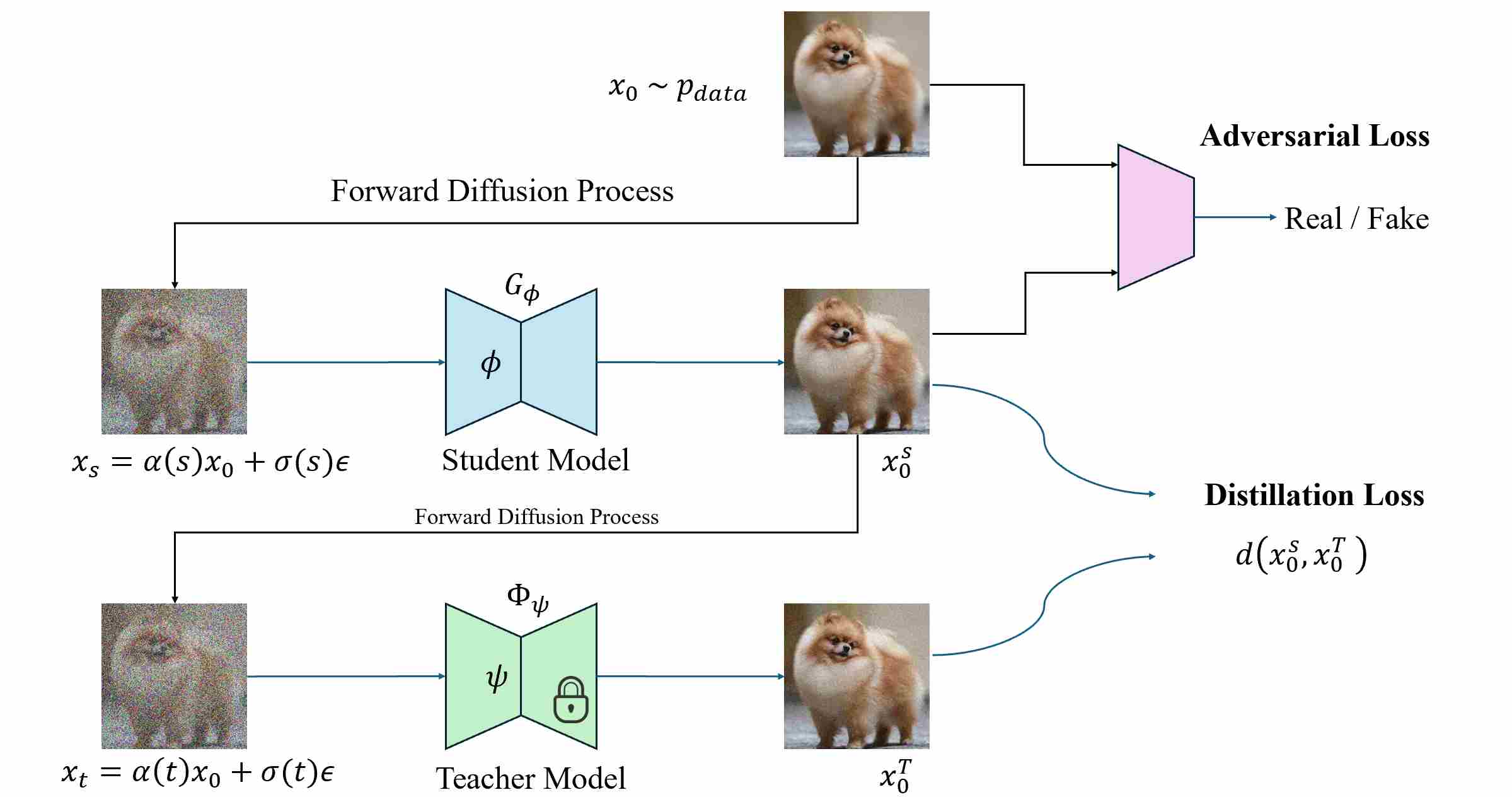
During training, let $x_0 \sim p_{\text{data}}$.

• Step 1: utilize forward diffusion process to add noise to clean image $x_0$.

  \[x_s = \alpha(s)x_0 + \sigma(s)\epsilon ,\qquad \epsilon \sim \mathcal N(0,I).\]

  where $0 < s \leq K $.

• step 2: The student first performs a s-step denoising:

  \[x_0^{S}=G_\phi(x_s; s\to 0)\]

  This represents the image the student would produce during inference.

• step 3: Instead of drawing real data $x_0$ again from the dataset, ADD reuses the student’s own output $x_0^{S}$ and applies forward diffusion:

  \[x_t = \alpha(t) x_0^{S} + \sigma(t)\epsilon^{'} , \qquad \epsilon^{'} \sim \mathcal N(0,I).\]

  where $0 < t \leq T $. This design is crucial—the teacher is conditioned on the student’s current distribution rather than on real data. By doing so, the teacher supervises exactly the domain that the student will visit at inference time, forming a closed-loop, on-policy distillation process.

• step 4: The teacher diffusion model, typically a pretrained DDIM or PF-ODE sampler, now starts from $x_t$ and performs full multi-step denoising:

  \[x_0^{T}=\Phi_{\text{teacher}}(x_t;\,t\to 0),\]

  yielding a high-quality reconstruction of what that noisy sample should look like under the teacher’s diffusion dynamics.

• step 5: The pair $(x_0^{S},,x_0^{T})$ defines the distillation target, while an adversarial discriminator evaluates realism relative to real data $x_0 \sim p_{\text{data}}$.

At inference, only the student is used: one forward pass from Gaussian noise $x_T$ directly yields $x_0^S$. The teacher is entirely discarded.

9.3 Distribution Matching Distillation

Distribution Matching Distillation (DMD) ¹¹ introduces a more principled and stable formulation. Rather than relying on an explicit discriminator, DMD enforces that the distribution of samples produced by a student one-step generator matches the distribution implicitly represented by the teacher diffusion model. This approach reframes diffusion distillation as a distribution-level alignment problem, bridging the gap between likelihood-based diffusion modeling and sample-based generative matching.

9.3.1 Motivation – Beyond Adversarial Alignment

Instead of forcing a student to mimic the teacher’s noise→image mapping point-by-point (which is expensive and brittle), Distribution Matching Distillation (DMD) trains a one-step generator so that its distribution of outputs becomes indistinguishable from the data distribution learned by the base diffusion model. We do not require the output of the student model to be exactly the same as that of the teacher model for each sample; instead, we are more concerned that the output distribution of the student model should be as consistent as possible with that of the teacher model.

To make it feasible, the DMD design consists of three network structures.

• Base (real) denoiser $\mu_{\text{base}}(x_t,t)$: a pretrained diffusion model (EDM or Stable Diffusion) used as a frozen score estimator for the diffused real distribution.

• One-step generator $G_\theta(z)$: same architecture as the denoiser but no time input; initialized from the base model’s weights (mean-prediction form in the paper, works identically with $\epsilon$-prediction).

• Fake (dynamic) denoiser $\mu_{\phi}^{\text{fake}}(x_t,t)$: trainable denoiser that continuously fits the current student distribution (used to compute the fake score).

9.3.2 Principle and Formulation

Two ingredients make DMD work, The final generator loss consists of two components

• Distribution-Matching Loss. which is used to minimize the student output distribution ($p_{\text{fake}}$) and the teacher output distribution ($p_{\text{real}}$).

  \[D_{\mathrm{KL}}\big(p_{\text{fake}}\ |\ p_{\text{real}}\big)\;=\;\mathbb{E}_{x\sim p_{\text{fake}}}\big[\log p_{\text{fake}}(x)-\log p_{\text{real}}(x)\big],\]

• Regression Loss. The KL gradient above is well-behaved at moderate–high noise but can get unreliable at very low noise (real density nearly zero off-manifold). Also, scores are invariant to scaling of the density, which can invite mode collapse/dropping. DMD therefore adds a tiny amount of paired supervision: precompute a small set of (noise, multi-step output) pairs $(z,y)$ from the base model via a deterministic ODE sampler, and minimize

  \[\mathcal L_{\text{reg}}=\mathbb{E}_{(z,y)}\,\text{LPIPS}\big(G_\theta(z),\,y\big).\]

  where $\text{LPIPS}$ ¹² is an abbreviation for Learned Perceptual Image Patch Similarity, a learned deep feature–based metric that measures perceptual similarity between two images, capturing human visual judgment more accurately than pixel-wise distances or conventional perceptual losses.

The final generator loss is

The following figure shows optimizing various objectives starting from the initial state leads to different outcomes.

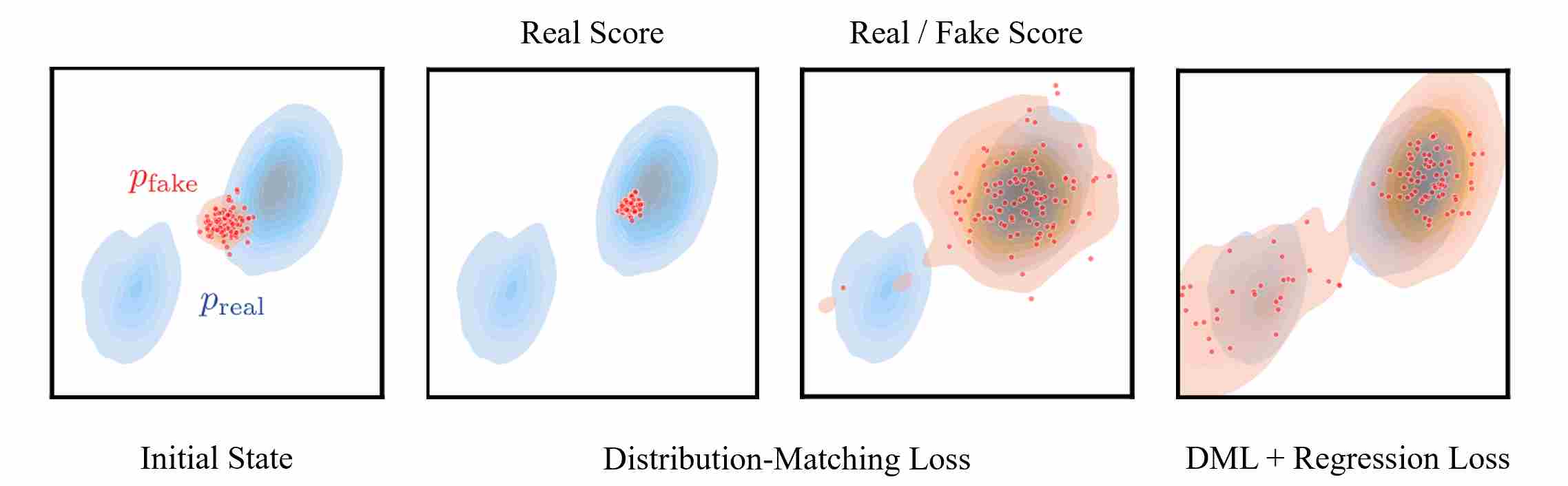
9.3.3 The core objective: KL Divergence

DMD minimizes

with $x=G_\theta(z),\ z\sim\mathcal N(0,I)$. Differentiating w.r.t. $\theta$ using reparameterization gives

where $s(\cdot)=\nabla_x \log p(\cdot)$ is the score. Intuition: $s_{\text{real}}$ pushes samples toward real modes; $-s_{\text{fake}}$ “spreads” samples away from spurious fake modes. The generator update thus follows (fake − real).

However, two issues arise in the image space:

• Scores may be undefined where the other distribution has zero density, that’s because at the very beginning, there is almost no overlap between $p_{\text{fake}}$ and $p_{\text{real}}$, according to the score definition

  \[s_{\text{real}} = \nabla_x \log p_{\text{real}}(x) = \frac{\nabla_x p_{\text{real}}(x)}{p_{\text{real}}(x)}\]

  since $x\sim p_{\text{fake}}$, makes $p_{\text{real}}(x) = 1$ for most area.

• We don’t know the exact distribution of $p_{\text{real}}$ and $p_{\text{fake}}$.

Diffusion models estimate scores of diffused distributions, not the raw data distribution. The fix is to work in diffusion space: perturb $x$ with Gaussian noise to obtain \(x_t\sim q_t(x_t \mid x)=\mathcal N(\alpha_t x,\sigma_t^2 I)\), where supports overlap and denoisers approximate the corresponding scores.

Using mean-prediction form ³, the scores at time $t$ are

Then the distribution-matching update becomes

with a carefully chosen time weight $w_t$ to normalize gradient magnitudes across noise levels.

9.3.4 How the "fake denoiser" is trained

Because the student’s output distribution keeps evolving, DMD trains a dynamic fake denoiser \(\mu_{\phi}^{\text{fake}}\) to track the current fake distribution. Training uses a standard diffusion denoising loss

where $x_0$ is the (stop-grad) student output that was just diffused to form $x_t$. This keeps $\mu_{\phi}^{\text{fake}}$ on-support for the fake distribution, so its score is numerically stable and informative for the generator update.

9.4 Score Distillation

10. Flow Matching: A New Paradigm for Fast Sampling

In this section, we provide a concise overview of Flow Matching (FM) as a novel training paradigm for fast generative sampling. A detailed and technical analysis of flow matching will be presented in a separate dedicated article.

10.1 From Numerical Acceleration to Training-Level Acceleration

The first two families of acceleration methods reviewed earlier—high-order ODE solvers (Chapter 7) and distillation-based acceleration (Chapter 8 and Chapter 9)—primarily address how to make an already-trained diffusion model generate faster.

They either 1). design more accurate numerical integrators to approximate the same diffusion ODE in fewer steps, or 2). learn a student network that imitates the teacher’s multi-step trajectory within one or a few denoising passes.

By contrast, Flow Matching does not rely on an existing teacher model or on post-hoc solver improvements. Instead, it redefines the training objective itself—learning a continuous vector field that transports samples from noise to data along the most efficient and smooth path. In other words, rather than speeding up sampling after training, FM builds the notion of efficiency into the training dynamics.

10.2 The Core Idea: Learning the Optimal Transport Flow

At its heart, flow matching treats generation as learning an ordinary differential equation

whose trajectories deterministically transform the noise distribution into the data distribution. Unlike diffusion training, which learns a stochastic denoising score field and relies on thousands of discretization steps, flow matching directly learns the deterministic transport velocity between the two distributions.

The essential insight is that the geometry of this learned flow field determines sampling speed: if the field forms a straight and low-curvature path from noise to data, the ODE can be integrated in far fewer steps without deviating from the target manifold. Thus, FM aims to find the shortest and flattest path—a “geodesic” in distribution space—rather than merely replicating the stochastic diffusion trajectory.

11. References