When discussing the stability of diffusion model training, much of the focus often falls on noise schedules, loss weighting strategies, or optimization tricks (Please refer our post). While these aspects are undeniably important, an equally critical — yet sometimes underemphasized — factor is the choice of network architecture itself. The structure of the model fundamentally determines how signals, gradients, and conditioning information propagate across different noise levels, and whether the training process converges smoothly or collapses into instability.

1. Why Architecture Matters for Stability

Network architecture is more than a vessel for function approximation in diffusion models — it is the key component that determines whether training succeeds or fails.

1.1 Gradient Flow, Conditioning, and Stability

Diffusion models are trained under extreme conditions: inputs span a spectrum from nearly clean signals to pure Gaussian noise. This makes them particularly sensitive to how gradients are normalized, how residuals accumulate, and how skip connections or attention layers interact with noisy features.

• Improper gradient flow can cause exploding updates at low-noise regimes or vanishing signals at high-noise regimes.
• Conditioning pathways (e.g., cross-attention for text or multimodal prompts) introduce additional sensitivity, as misaligned normalization or unbalanced skip pathways can destabilize learning.

Architectural innovations such as GroupNorm, AdaLN-Zero, and preconditioning layers have been specifically introduced to address these gradient stability issues, ensuring that the network remains trainable across a wide dynamic range of noise.

1.2 Balancing Capacity vs. Robustness

A second challenge lies in the tension between capacity (the ability of the architecture to represent complex distributions) and robustness (the ability to generalize under noisy, unstable conditions).

• Early U-Net designs offered robustness through simplicity and skip connections, but limited capacity for scaling.
• Transformer-based diffusion models (DiT, MMDiT-X) introduced massive representational power, but at the cost of more fragile training dynamics.
• Newer architectures explore hybrid or modular designs — combining convolutional inductive biases, residual pathways, and attention — to find a stable equilibrium between these two competing goals.

1.3 Architecture–Noise Schedule Coupling

Finally, the stability of diffusion training cannot be isolated from the noise schedule. Architectural design interacts tightly with how noise levels are distributed and parameterized:

• A model with time-dependent normalization layers may remain stable under variance-preserving schedules but collapse under variance-exploding ones.
• EDM (Elucidated Diffusion Models) highlight that architecture and preconditioning must be co-designed with the training noise distribution, rather than treated as independent modules.

This coupling implies that progress in diffusion training stability comes not only from better solvers or schedules, but from holistic architectural design that accounts for gradient dynamics, representation capacity, and their interplay with noise parameterization.

2. Evolution of Diffusion Architectures

The architectural journey of diffusion models mirrors the evolution of deep learning itself: from simple convolutional backbones to large-scale Transformers, and now toward specialized multi-modal and efficiency-driven designs. Each stage has sought to reconcile two opposing pressures — increasing representational power while preserving training stability. In this section, we trace this trajectory across six key phases.

2.1 Classical U-Net Foundations

The U-Net architecture ¹ is the canonical backbone of early diffusion models such as DDPM ². Although originally proposed for biomedical image segmentation ¹ , its encoder–decoder structure with skip connections turned out to be perfectly suited for denoising across different noise levels. The elegance of U-Net lies not only in its symmetry, but also in how it balances global context extraction with local detail preservation. A typical unet structure applied to the training of diffusion models is as follows

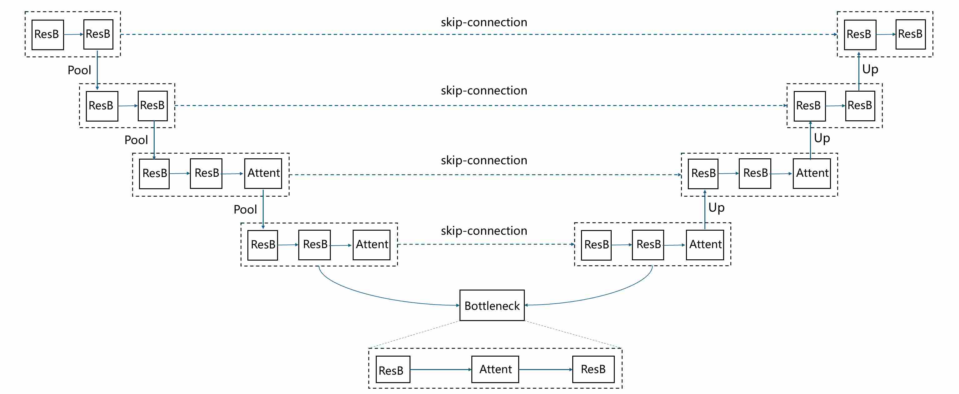
where ResB represents residual block, who consists of multiple “norm-act-conv2d” layers. Attent represents self-Attention block.

2.1.1 Encoder: From Local Features to Global Context

The encoder path consists of repeated convolutional residual blocks and downsampling operations (e.g., strided convolutions or pooling). As the spatial resolution decreases and channel width expands, the network progressively shifts its representational emphasis:

• High-resolution feature maps (early layers) capture fine-grained local structures — edges, textures, and small patterns that are critical when denoising images at low noise levels.
• Low-resolution feature maps (deeper layers) aggregate global context — object shapes, spatial layout, and long-range dependencies. This is especially important at high noise levels, when much of the local structure has been destroyed and only global semantic cues can guide reconstruction.

Thus, the encoder effectively builds a multi-scale hierarchy of representations, transitioning from local to global as resolution decreases.

2.1.2 Bottleneck: Abstract Representation

At the center lies the bottleneck block, where feature maps have the smallest spatial size but the largest channel capacity. This stage acts as the semantic aggregator:

• It condenses the global context extracted from the encoder.
• It often includes attention layers (in later refinements) to explicitly model long-range interactions. In the classical U-Net used by DDPM, the bottleneck is still purely convolutional, yet it already plays the role of a semantic “bridge” between encoding and decoding.

2.1.3 Decoder: Reconstructing Local Detail under Global Guidance

The decoder path mirrors the encoder, consisting of upsampling operations followed by convolutional residual blocks. The role of the decoder is not merely to increase resolution, but to inject global semantic context back into high-resolution predictions:

• Upsampling layers expand the spatial resolution but initially lack fine detail.
• Skip connections from the encoder reintroduce high-frequency local features (edges, boundaries, textures) that would otherwise be lost in downsampling.
• By concatenating or adding these skip features to the decoder inputs, the network fuses global context (from low-res encoder features) with local precision (from high-res encoder features).

This synergy ensures that the denoised outputs are both semantically coherent and visually sharp.

2.1.4 Timestep Embedding and Conditioning

Unlike the U-Net’s original role in segmentation, a diffusion U-Net must also be conditioned on the diffusion timestep $t$, since the network’s task changes continuously as noise levels vary. In the classical DDPM implementation, this conditioning is realized in a relatively simple but effective way:

1. Sinusoidal embedding. Each integer timestep $t$ is mapped to a high-dimensional vector using sinusoidal position encodings (analogous to Transformers), ensuring that different timesteps are represented as distinct, smoothly varying signals.

2. MLP transformation. The sinusoidal embedding is passed through a small multilayer perceptron (usually two linear layers with a SiLU activation) to produce a richer time embedding vector $\mathbf{z}_t$.

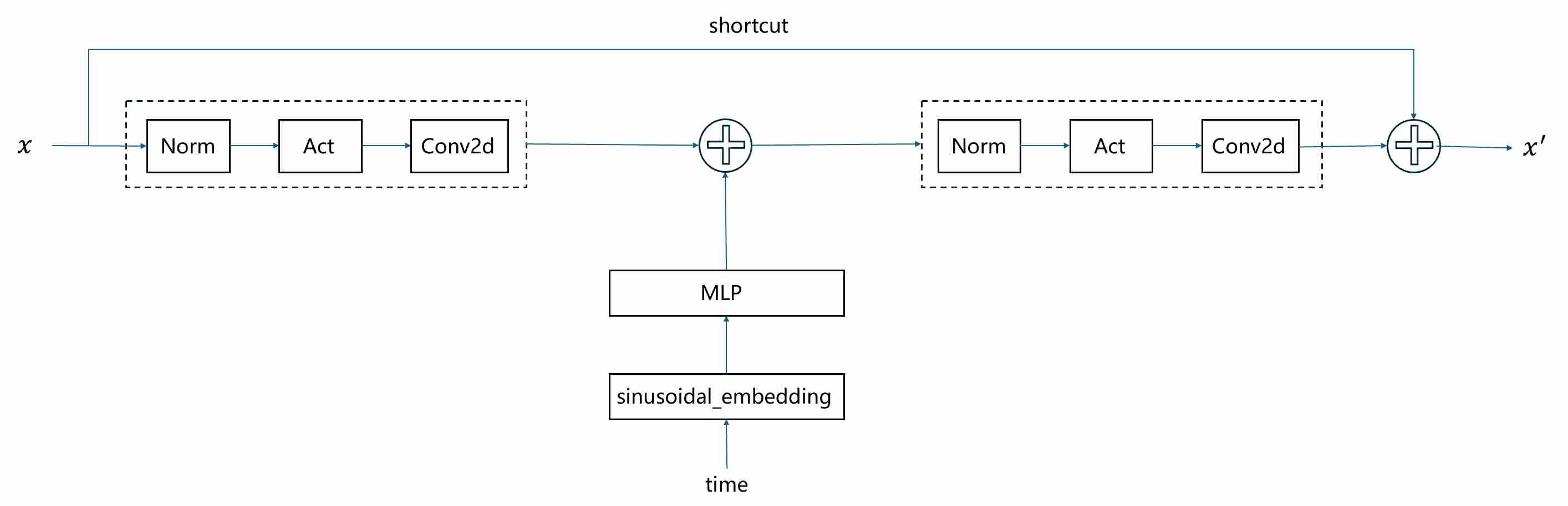
3. Additive injection into residual blocks. In every residual block of the U-Net, $\mathbf{z}_t$ is projected to match the number of feature channels and then added as a bias term to the intermediate activations (typically after the first convolution).

This additive conditioning allows each residual block to adapt its computation based on the current noise level, without introducing extra normalization or complex modulation. The following figure shows the way how to inject timestep $t$ in each residual block.

2.1.5 Why U-Net Works Well for Diffusion

In diffusion training, inputs vary drastically in signal-to-noise ratio:

• At low noise levels, local details still survive; skip connections ensure these details propagate to the output.
• At high noise levels, local detail is destroyed; the decoder relies more on global semantics from the bottleneck.
• Across all levels, the encoder–decoder interaction guarantees that both local fidelity and global plausibility are preserved.

This explains why U-Nets became the default backbone: their multi-scale design matches perfectly with the multi-scale nature of noise in diffusion models. Later improvements (attention layers, latent-space U-Nets, Transformer backbones) all build upon this foundation, but the core idea remains: stability in diffusion training emerges from balanced local–global feature fusion.

2.2 ADM Improvements (Ablated Diffusion Models)

While the classical U-Net backbone of DDPM demonstrated the feasibility of diffusion-based generation, it was still limited in stability and scalability. In the landmark work “Diffusion Models Beat GANs on Image Synthesis” ³, the authors performed extensive ablations to identify which architectural and training choices were critical at ImageNet scale. The resulting recipe is commonly referred to as ADM (Ablated Diffusion Models). Rather than introducing a single new module, ADM represents a carefully engineered upgrade to the baseline U-Net, designed to balance capacity, conditioning, and stability.

2.2.1 Scaling the U-Net: Wider Channels and Deeper Residual Blocks

The most straightforward but highly effective change was scaling up the model. The ADM UNet is significantly larger than the one used in the original DDPM paper.

• Wider Channels: The base channel count was increased (e.g., from 128 to 256), and the channel multipliers for deeper layers were adjusted, resulting in a much wider network.
• More Residual Blocks: The number of residual blocks per resolution level was increased, making the network deeper.

Why it helps: A larger model capacity allows the network to learn more complex and subtle details of the data distribution, leading to a direct improvement in sample fidelity.

2.2.2 Multi-Resolution Self-Attention

While DDPM’s UNet used self-attention, it was typically applied only at a single, low resolution (e.g., 16x16). ADM recognized that long-range dependencies are important at various scales.

In ADM, Self-attention blocks were added at multiple resolutions (e.g., 32x32, 16x16, and 8x8). Additionally, the number of attention heads was increased.

• Attention at higher resolutions (32x32) helps capture relationships between medium-sized features and textures;
• Attention at lower resolutions (8x8) helps coordinate the global structure and semantic layout of the image.

Why it helps: This multi-scale approach gives the model a more holistic understanding of the image, preventing structural inconsistencies and improving overall coherence.

2.2.3 Conditioning via Adaptive Group Normalization (AdaGN)

This is arguably the most significant architectural contribution of ADM. It fundamentally changes how conditional information (like timesteps and class labels) is integrated into the network.

• In DDPM: The time embedding was processed by an MLP and then simply added to the feature maps within each residual block. This acts as a global bias, which is a relatively weak form of conditioning.

• In ADM (AdaGN) ⁴: The model learns to modulate the activations using the conditional information. The process is as follows: a). The timestep embedding and the class embedding (for class-conditional models) are combined into a single conditioning vector; b). This vector is passed through a linear layer to predict two new vectors: a scale ($\gamma$) and a shift ($\beta$) parameter for each channel. c). Within each residual block, the feature map undergoes Group Normalization, and then its output is modulated by these predicted parameters.

Why it helps: Modulation is a much more powerful mechanism than addition. It allows the conditional information to control the mean and variance of each feature map on a channel-by-channel basis. This gives the model fine-grained control over the generated features, dramatically improving its ability to adhere to the given conditions (i.e., generating a specific class at a specific noise level).

2.2.4 BigGAN-inspired Residual Blocks for Up/Downsampling

ADM also identifies that the choice of downsampling and upsampling operations affects stability.

• In DDPM: Downsampling might be a simple pooling or strided convolution, and upsampling might be a standard upsample layer followed by a convolution.
• In ADM: The upsampling and downsampling operations were integrated into specialized residual blocks, a design inspired by the highly successful BigGAN architecture ⁵. This ensures that information flows more smoothly as the resolution changes, minimizing information loss.

It favors strided convolutions for downsampling and nearest-neighbor upsampling followed by convolution for upsampling.

Why it helps: This leads to better preservation of features across different scales, contributing to sharper and more detailed final outputs.

2.2.5 Rescaling of Residual Connections

For very deep networks, it’s crucial to maintain well-behaved activations. ADM introduced a simple but effective trick: The output of each residual block was scaled by a constant factor of 1/${\sqrt{2}}$ before being added back to the skip connection.

Why it helps: This technique helps to balance the variance contribution from the skip connection and the residual branch, preventing the signal from exploding in magnitude as it passes through many layers. This improves training stability for very deep models.

2.2.6 Why ADM Matters for Stability

Relative to the classical DDPM U-Net, in conclusion, the ADM UNet is a masterclass in architectural refinement. By systematically enhancing every major component—from its overall scale to the precise mechanism of conditional injection—it provided the powerful backbone necessary for diffusion models to finally surpass GANs in image synthesis quality.

2.3 Latent U-Net: The Efficiency Revolution with Stable Diffusion and SDXL

While the ADM architecture (Section 2.2) marked the pinnacle of pixel-space diffusion models, achieving state-of-the-art quality by meticulously refining the U-Net, it faced a significant and inherent limitation: computational cost. Training and running diffusion models directly on high-resolution images (e.g., 512x512 or 1024x1024) is incredibly demanding in terms of both memory and processing power. The U-Net must process massive tensors at every denoising step, making the process slow and resource-intensive.

The introduction of Latent Diffusion Models (LDMs) ⁶, famously realized in Stable Diffusion, proposed a revolutionary solution: instead of performing the expensive diffusion process in the high-dimensional pixel space, why not perform it in a much smaller, perceptually equivalent latent space? This insight effectively decouples the task of perceptual compression from the generative learning process, leading to a massive leap in efficiency and accessibility.

2.3.1 The Core Idea: Diffusion in a Compressed Latent Space

The training architecture of LDM is a two-stage process.

Stage 1: Perceptual Compression. A powerful, pretrained Variational Autoencoder (VAE) is trained to map high-resolution images into a compact latent representation and back. The encoder, $E$, compresses an image x into a latent vector $z = E(x)$. The decoder, $D$, reconstructs the image from the latent, \(\tilde x = D(z)\). Crucially, this is not just any compression; it is perceptual compression, meaning the VAE is trained to discard high-frequency details that are imperceptible to the human eye while preserving critical semantic and structural information.

Stage 2: Latent Space Diffusion. Instead of training a U-Net on images x, we train it on the latent codes $z$. The forward diffusion process adds noise to $z$ to get $z_t$, and the U-Net’s task is to predict the noise in this latent space.

The impact of this shift is dramatic. A 512x512x3 pixel image (786,432 dimensions) can be compressed by the VAE into a 64x64x4 latent tensor (16,384 dimensions)—a 48x reduction in dimensionality. The U-Net now operates on these much smaller tensors, enabling faster training and significantly lower inference requirements.

The full generative (inference) process for a text-to-image model like Stable Diffusion is as follows:

• Stage 1: Text Prompt $\to$ Text Encoder $\to$ Conditioning Vector $c$.
• Stage 2: Random Noise $z_T$ $\to$ U-Net Denoising Loop in Latent Space, conditioned on $c$ $\to$ Clean Latent \(z_0\).
• Stage 3: Clean Latent $z_0$ $\to$ VAE Decoder $\to$ Final Image $x$.

2.3.2 Architectural Breakdown of the Latent U-Net

While the Latent U-Net, exemplified by Stable Diffusion, inherits its foundational structure from the ADM architecture (i.e., a U-Net with residual blocks and multi-resolution self-attention), it introduces several profound modifications. These are not mere tweaks but fundamental redesigns necessary to operate efficiently in a latent space and to handle the sophisticated conditioning required for text-to-image synthesis.

Conditioning Paradigm Shift: From Global AdaGN to Localized Cross-Attention

This is the most critical evolution from the ADM architecture. ADM perfected conditioning for global, categorical information (like a single class label), whereas Stable Diffusion required a mechanism for sequential, localized, and compositional information (a text prompt).

• ADM’s Approach (Global Conditioning): ADM injected conditions (time embedding, class embedding) via adaptive normalization (AdaGN/FiLM): A single class embedding vector is combined with the time embedding. This unified vector is then projected to predict scale and shift parameters that modulate the entire feature map within a ResBlock. Limitation: This is an “all-at-once” conditioning signal. The network knows it needs to generate a “cat,” and this instruction is applied globally across all spatial locations. It cannot easily handle a prompt like “a cat sitting on a chair,” because the conditioning signal for “cat” and “chair” cannot be spatially disentangled.

• Latent U-Net’s Approach (Localized Conditioning): Latent U-Nets instead integrate text tokens (from a frozen text encoder, e.g., CLIP) using cross-attention at many/most resolutions: Instead of modulating activations, the U-Net directly incorporates the text prompt’s token embeddings at multiple layers. A text encoder (e.g., CLIP) first converts the prompt “a cat on a chair” into a sequence of token embeddings: [, a, cat, on, a, chair, ].

  These embeddings form the Key (K) and Value (V) for the cross-attention mechanism. The U-Net’s spatial features act as the Query (Q). At each location in the feature map, the Query can “look at” the sequence of text tokens and decide which ones are most relevant. A region of the feature map destined to become the cat will learn to place high attention scores on the “cat” token, while a region for the chair will attend to the “chair” token.

  \[\begin{aligned} \small & \text{Attn}(Q,\,K,\,V)=\text{softmax}(QK^T/\sqrt{d})V,\quad \\[10pt] & Q=\text{latent features},\quad K,V=\text{text tokens} \end{aligned}\]

The Division of Labor: Self-Attention vs. Cross-Attention

The modern Latent U-Net block now has a clear and elegant division of labor:

• Self-Attention: capture long-range dependencies and ensure global structural/semantic consistency. Convolutions and skip connections excel at local detail, but struggle to enforce coherence across distant regions. Self-attention fills this gap. Self-Attention typically only at low-resolution stages (e.g., 16×16 or 8×8).

• Cross-Attention: enable multimodal alignment, projecting language semantics onto spatial locations. Coarse-scale cross-attn controls global layout, style, and subject placement. Fine-scale cross-attn refines local textures, materials, and fine details.

This dual-attention design is profoundly more powerful than ADM’s global conditioning, enabling the complex compositional generation we see in modern text-to-image models. Cross-Attention usually at multiple scales, often after each residual block.

Adapting the Training Objective for Latent Space: $\epsilon$-prediction vs. $v$-prediction

Another key adaptation that makes training deep and powerful U-Nets in latent space more robust and effective is the choice of objective.

We have discussed four common prediction targets to train diffusion models (post). Through analysis and comparison, we found that $v$-prediction has the best stability, this led LDM to shift towards using $v$ instead of $\epsilon$ to achieve more stable training results.

Perceptual Weighting in Latent Space

In Latent Diffusion Models, diffusion is not trained directly in pixel space but in the latent space of a perceptual autoencoder (a VAE). The latent representation is much smaller (e.g., 64×64×4 for a 512×512 image) and is designed to preserve perceptually relevant information.

However, if we train the diffusion model with a plain mean squared error (MSE) loss on the latent vectors, you implicitly treat all latent dimensions and spatial positions as equally important. In practice:

• Some latent channels carry critical perceptual information (edges, textures, semantics).
• Other channels encode redundant or imperceptible details.

Without adjustment, the diffusion model may spend too much gradient budget on parts of the latent space that have little impact on perceptual quality. Perceptual weighting introduces a weighting factor $w(z)$ into the diffusion loss, so that errors in perceptually important latent components are emphasized:

There are different ways to define $w(z)$:

1. Channel-based weighting from the VAE

   • Estimate how much each latent channel contributes to perceptual fidelity (e.g., by measuring sensitivity of the VAE decoder to perturbations in that channel).
   • Assign larger weights to channels that strongly affect the decoded image.

2. Feature-based weighting (perceptual features)

   • Decode the latent $z$ back to image space $x=D(z)$.
   • Extract perceptual features $\phi(x)$ (e.g., from a VGG network or LPIPS).
   • Estimate how sensitive these features are to changes in $z$. Latent dimensions with high sensitivity get higher weights.

3. Static vs. adaptive weighting

   • Static: Precompute a set of per-channel weights (averaged over the dataset).
   • Adaptive: Compute weights on the fly per sample or per timestep using Jacobian-vector product tricks.

In summary:

• Focus on perceptual quality: Gradients are concentrated on latent components that most affect the decoded image quality.
• Suppress irrelevant gradients: Channels that mostly encode imperceptible high-frequency noise are downweighted.
• More stable training: The denoiser learns where its predictions matter most, reducing wasted updates and improving convergence.

2.3.3 Evolution to SDXL: Refining the Latent U-Net Formula

While Stable Diffusion models 1.x and 2.x established the power of the Latent Diffusion paradigm, Stable Diffusion XL (SDXL) ⁷ represents a significant architectural leap forward. It is not merely a larger model but a systematically re-engineered system designed to address the core limitations of its predecessors, including native resolution, prompt adherence, and aesthetic quality. The following sections provide a detailed technical breakdown of the key architectural innovations in SDXL.

A Two-Stage Cascade Pipeline: The Base and Refiner Models

To achieve the highest level of detail and aesthetic polish, SDXL introduces an optional but highly effective two-stage generative process, employing two distinct models.

• Stage 1: The Base Model
  • Architecture: This is the main, large U-Net with the dual text encoder system described above.
  • Function: It performs the bulk of the denoising process, starting from pure Gaussian noise and running for a majority of the sampling steps. Its primary responsibility is to establish a strong global composition, accurate color harmony, and correct semantic content. The output is a high-quality latent representation that is structurally sound but may lack the finest high-frequency details.
• Stage 2: The Refiner Model
  • Architecture: The refiner is another Latent Diffusion Model, architecturally similar to the base but specifically optimized for a different task.
  • Specialized Training: The refiner is trained exclusively on images with a low level of noise. This makes it an “expert” at high-fidelity rendering and detail injection, rather than coarse-to-fine generation.
  • Function: It takes the latent output from the base model and performs a small number of final denoising steps. In this low-noise regime, it focuses on sharpening details, correcting minor artifacts, and adding intricate textures (e.g., skin pores, fabric weaves).

Impact: This ensemble-of-experts approach allows for a division of labor. The base model ensures robust composition, while the refiner specializes in aesthetic finalization. The result is an image that benefits from both global coherence and local, high-frequency richness, achieving a level of quality that is difficult for a single model to produce consistently.

A Substantially Larger and More Robust U-Net Backbone

The most apparent upgrade in SDXL is its massively scaled-up U-Net, which serves as the core of the base model. This expansion goes beyond a simple increase in parameter count to include strategic design choices.

• Increased Capacity: The SDXL base U-Net contains approximately 2.6 billion parameters, a nearly threefold increase compared to the ~860 million parameters of the U-Net in SD 1.5. This additional capacity is crucial for learning the more complex and subtle features required for high-resolution 1024x1024 native image generation.

• Deeper and Wider Architecture: The network’s depth (number of residual blocks) and width (channel count) have been significantly increased. Notably, the channel count is expanded more aggressively in the middle blocks of the U-Net. These blocks operate on lower-resolution feature maps (e.g., 32x32) where high-level semantic information is most concentrated. By allocating more capacity to these semantic-rich stages, the model enhances its ability to reason about object composition and global scene structure, directly mitigating common issues like malformed anatomy (e.g., extra limbs) seen in earlier models at high resolutions.

• Refined Attention Mechanisms: The distribution and configuration of the attention blocks (both self-attention and cross-attention) across different resolution levels were re-evaluated and optimized. This ensures a more effective fusion of spatial information (from the image features) and semantic guidance (from the text prompt) at all levels of abstraction.

Impact: This fortified U-Net backbone is the primary reason SDXL can generate coherent, detailed, and aesthetically pleasing images at a native 1024x1024 resolution, a feat that was challenging for previous versions without significant post-processing or specialized techniques.

The Dual Text Encoder: A Hybrid Approach to Prompt Understanding

Perhaps the most innovative architectural change in SDXL is its departure from a single text encoder. SDXL employs a dual text encoder strategy to achieve a more nuanced and comprehensive understanding of user prompts.

• OpenCLIP ViT-bigG: This is the larger of the two encoders and serves as the primary source of high-level semantic and conceptual understanding. Its substantial size allows it to grasp complex relationships, abstract concepts, and the overall sentiment or artistic intent of a prompt (e.g., “a majestic castle on a hill under a starry night”).

• CLIP ViT-L: The second encoder is the standard CLIP model used in previous Stable Diffusion versions. It excels at interpreting more literal, granular, and stylistic details in the prompt, such as specific objects, colors, or artistic styles (e.g., “a red car,” “in the style of Van Gogh”).

Mechanism of Fusion: During inference, the input prompt is processed by both encoders simultaneously. The resulting sequences of token embeddings are then concatenated along the channel dimension before being fed into the U-Net’s cross-attention layers. This combined embedding provides the U-Net with a richer, multi-faceted conditioning signal.

Impact: This hybrid approach allows SDXL to reconcile two often competing demands: conceptual coherence and stylistic specificity. The model can understand the “what” (from ViT-L) and the “how” (from ViT-bigG) of a prompt with greater fidelity, leading to superior prompt adherence and the ability to generate complex, well-composed scenes that match the user’s intent more closely.

Micro-Conditioning for Resolution and Cropping Robustness

SDXL introduces a subtle yet powerful form of conditioning that directly addresses a common failure mode in generative models: sensitivity to image aspect ratio and object cropping.

• The Problem: Traditional models are often trained on square-cropped images of a fixed size. When asked to generate images with different aspect ratios, they can struggle, often producing unnatural compositions or cropped subjects.

• SDXL’s Solution: During training, the model is explicitly conditioned on several metadata parameters in addition to the text prompt:

  • original height and original width: The dimensions of the original image before any resizing or cropping.
  • crop top and crop left: The coordinates of the top-left corner of the crop.
  • target height and target width: The dimensions of the final generated image.

Mechanism of Injection: These scalar values are converted into a fixed-dimensional embedding vector. This vector is then added to the sinusoidal time embedding before being passed through the AdaGN layers of the U-Net’s residual blocks.

Impact: By making the model “aware” of the resolution and framing context, SDXL learns to generate content that is appropriate for the specified canvas. This significantly improves its ability to handle diverse aspect ratios and dramatically reduces instances of unwanted cropping, leading to more robust and predictable compositional outcomes.

2.4 Transformer-based Designs

While latent U-Nets (Section 2.3) significantly improved efficiency and multimodal conditioning, they still retained convolutional inductive biases and hierarchical skip pathways. Due to the success of Transformers ⁸ in large-scale NLP tasks, the next stage in the evolution of diffusion architectures explores whether Transformers can serve as the primary backbone for diffusion models. This marks a decisive shift from UNET-dominated designs to Transformer-native backbones, most notably exemplified by the Diffusion Transformer (DiT) ⁹ family and its successors.

2.4.1 Motivation for Transformer Backbones

Convolution-based U-Nets provide strong locality and translation invariance, but they impose rigid inductive biases:

• Locality and Global Context: Convolutions capture local patterns well but require deep hierarchies to model long-range dependencies. U-Nets solve this partially through down/upsampling and skip connections, but global coherence still relies on explicit attention layers carefully placed at coarse scales.

  Transformers, by contrast, model all-pair interactions directly via attention, making them natural candidates for tasks where global semantics dominate.

• Benefit from Scaling laws: Recent work shows that Transformers scale more predictably with dataset and parameter count, whereas CNNs saturate earlier. Diffusion training, often performed at very large scales, benefits from architectures that exhibit similar scaling behavior.

• Unified multimodal processing.: Many diffusion models condition on text or other modalities. Transformers provide a token-based interface: both images (as patch embeddings) and text (as word embeddings) can be treated uniformly, simplifying multimodal alignment.

Thus, a Transformer-based backbone promises to simplify design and leverage established scaling laws, potentially achieving higher fidelity with cleaner training dynamics.

2.4.2 Architectural Characteristics of Diffusion Transformers

The Diffusion Transformer (DiT) proposed by Peebles & Xie (2022) was the first systematic exploration of replacing U-Nets with ViT-style Transformers for diffusion.

• Patch tokenization: Instead of convolutions producing feature maps, the input (pixels or latents) is divided into patches (e.g., 16×16), each mapped to a token embedding. This yields a sequence of tokens that a Transformer can process natively.
• Class and time conditioning: As in ADM, timestep and class embeddings are injected not by concatenation but by scale-and-shift modulation of normalization parameters. The different is that, instead of AdaGN, DiT uses Adaptive LayerNorm (AdaLN).
• Global self-attention: Unlike U-Nets, where attention is inserted at selected resolutions, DiT-style models apply self-attention at every layer. This uniformity eliminates the need to decide “where” to place global reasoning — it is omnipresent.
• Scalability: Transformers scale more gracefully with depth and width. With large batch training and data-parallelism, models like DiT-XL can be trained efficiently on modern accelerators.

DiT demonstrates that diffusion models do not require convolutional backbones. However, it also reveals that training Transformers for denoising is more fragile: optimization can collapse without careful normalization (AdaLN-Zero) and initialization tricks.

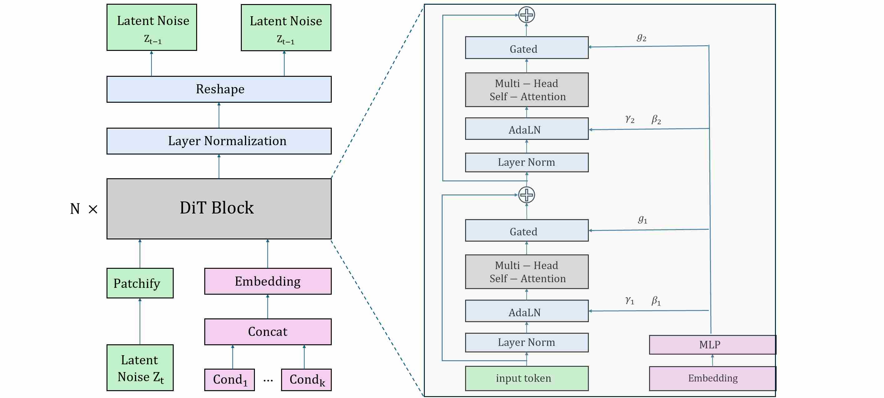
The Diffusion Transformer (DiT) architecture is as shown below.

2.4.3 Hybrid Designs: Marrying U-Net and Transformer Strengths

Pure Transformers are computationally expensive, especially at high resolutions. To balance efficiency and quality, several hybrid architectures emerged:

• U-Net with Transformer blocks — many models, including Stable Diffusion v2 and SDXL, interleave attention layers (which are Transformer sub-blocks) into convolutional U-Nets. This compromise preserves locality while still modeling long-range dependencies.

• Perceiver-style cross-attention. Conditioning (e.g., text embeddings) can be injected via cross-attention, a Transformer-native mechanism that naturally fuses multimodal tokens.

• MMDiT (Multimodal DiT) in Stable Diffusion 3. Here, both image latents and text tokens are treated as tokens in a single joint Transformer sequence. Queries, keys, and values are drawn from both modalities, enabling a fully symmetric text–image fusion mechanism without the asymmetry of U-Net cross-attention layers.

2.5 Extensions to Video and 3D Diffusion

The success of diffusion models on static images naturally prompted their extension to more complex, higher-dimensional data like video and 3D scenes. This required significant architectural innovations to handle the temporal dimension in video and the complex geometric representations of 3D objects, all while maintaining consistency and stability.

2.5.1 Video U-Net: Introducing the Temporal Dimension

The most direct way to adapt an image U-Net for video generation is to augment it with mechanisms for processing the time axis. This gave rise to the Spatio-Temporal U-Net.

Temporal Layers for Consistency

A video can be seen as a sequence of image frames, i.e., a tensor of shape (B, T, C, H, W). A standard 2D U-Net processes each frame independently, leading to flickering and temporal incoherence. To solve this, temporal layers are interleaved with the existing spatial layers:

• Temporal Convolutions: 3D convolution layers (e.g., with a kernel size of (3, 3, 3) for (T, H, W)) replace or supplement the standard 2D convolutions. This allows features to be aggregated from neighboring frames.
• Temporal Attention: This is the more powerful and common approach. After a spatial self-attention block that operates within each frame, a temporal self-attention block is added. In this block, a token at frame t attends to corresponding tokens at other frames (t-1, t+1, etc.). This explicitly models long-range motion and appearance consistency across the entire video clip.

Models like Stable Video Diffusion (SVD) build upon a pretrained image LDM and insert these temporal attention layers into its U-Net. By first training on images and then fine-tuning on video data, the model learns temporal dynamics while leveraging the powerful prior of the image model.

Conditioning on Motion

To control the dynamics of the generated video, these models are often conditioned on extra information like frames per second (FPS) or motion “bucket” IDs representing the amount of camera or object motion. This conditioning is typically injected alongside the timestep embedding, allowing the model to generate videos with varying levels of activity.

2.5.2 3D Diffusion: Generating Representations Instead of Pixels

Generating 3D assets is even more challenging due to the complexity of 3D representations (meshes, voxels, NeRFs) and the need for multi-view consistency. A breakthrough approach has been to use diffusion models to generate the parameters of a 3D representation itself, rather than rendering pixels directly.

Diffusion on 3D Gaussian Splatting Parameters

3D Gaussian Splatting (3D-GS) has emerged as a high-quality, real-time-renderable 3D representation. A scene is represented by a collection of 3D Gaussians, each defined by parameters like position (XYZ), covariance (scale and rotation), color (RGB), and opacity.

Instead of a U-Net that outputs an image, models like 3D-GS Diffusion use an architecture (often a Transformer) to denoise a set of flattened Gaussian parameters. The process works as follows:

1. Canonical Representation: A set of initial Gaussian parameters is created (e.g., a sphere or a random cloud).
2. Diffusion Process: Noise is added to this set of parameters (position, color, etc.) over time.
3. Denoising Network: A Transformer-based model takes the noisy parameter set and the conditioning signal (e.g., text or a single image) and predicts the clean parameters.
4. Rendering: Once the denoised set of Gaussian parameters is obtained, it can be rendered from any viewpoint using a differentiable 3D-GS renderer to produce a 2D image.

This approach elegantly separates the generative process (in the abstract parameter space) from the rendering process. By operating on the compact and structured space of Gaussian parameters, the model can ensure 3D consistency by design, avoiding the view-incoherence problems that plague naive image-space 3D generation.

2.6 Lightweight & Memory-Efficient Designs

While the trend has been towards ever-larger models like SDXL and DiT to push the boundaries of quality, a parallel and equally important line of research has focused on making diffusion models smaller, faster, and more accessible. The goal is to enable deployment on resource-constrained hardware like mobile phones and browsers, and to reduce the prohibitive costs of training and inference.

2.6.1 Core Strategies for Model Compression

Achieving efficiency requires a multi-pronged approach that combines architectural modifications with specialized training techniques.

Architectural Simplification

This involves designing a U-Net or Transformer that is inherently less computationally expensive.

• Shallow and Narrow Networks: The most straightforward method is to reduce the number of layers (depth) and the number of channels in each layer (width).
• Efficient Building Blocks: Replacing standard, costly operations with cheaper alternatives. For example, using depthwise separable convolutions instead of standard convolutions, or replacing full self-attention with more efficient variants like linear attention.
• Removing Redundant Blocks: Systematically ablating parts of a large model (e.g., removing attention blocks from the higher-resolution U-Net stages) to find a minimal-but-effective architecture.

Knowledge Distillation

This is a powerful training paradigm where a small “student” model is trained to mimic the behavior of a large, pretrained “teacher” model. In the context of diffusion, this is often done via Progressive Distillation ¹⁰. The student model is trained to predict the output of two steps of the teacher model in a single step, effectively halving the number of required sampling steps. This process can be applied iteratively to create models that generate high-quality images in just a few steps (e.g., 4-8 steps instead of 50).

2.6.2 Case Studies: MobileDiffusion and LightDiffusion

Several models exemplify these efficiency principles.

• MobileDiffusion: This work focuses on creating a text-to-image model that runs efficiently on mobile devices. It employs a highly optimized U-Net with a significantly reduced parameter count and FLOPs. The architectural choices are driven by hardware-aware design principles, favoring operations that are fast on mobile GPUs.

• LightDiffusion / TinySD: These models push the limits of compression. They often combine a heavily simplified U-Net architecture with knowledge distillation from a larger teacher model (like SDXL). For instance, a TinySD model might have only a fraction of the parameters of SD 1.5 but can produce surprisingly coherent results by learning the distilled output distribution of its teacher.

2.6.3 The Stability-Fidelity Trade-off

Designing lightweight models involves a fundamental trade-off. Smaller models have less capacity to capture the full complexity of the data distribution, which can lead to a reduction in sample quality, diversity, and prompt adherence. However, their smaller size and simpler architecture often result in a more stable and faster training process. The central challenge in this domain is to find novel architectures and training methods that push the Pareto frontier, achieving the best possible fidelity for a given computational budget. These efforts are crucial for the widespread democratization and practical application of diffusion model technology.

3. Stability-Oriented Architectural Designs

Training stability is a fundamental requirement for scaling diffusion models. While optimization strategies such as learning-rate schedules or variance weighting are important, the architecture itself largely determines whether gradients vanish, explode, or propagate smoothly across hundreds of layers. In diffusion models, two major architectural paradigms dominate: U-Net backbones (used in DDPM, ADM, Stable Diffusion) and Transformer backbones (DiT, MMDiT, SD3). These two paradigms embody different design philosophies, which in turn dictate distinct stabilization strategies.

3.1 Architectural Philosophies: U-Net vs. DiT

Before diving into specific mechanisms, we must first understand the high-level topological differences between U-Nets and DiTs. The very shape of these architectures dictates their inherent strengths, weaknesses, and, consequently, where the primary “pressure points” for stability lie.

3.1.1 U-Net Macro Topology

We have already covered most of the knowledge about the UNET structure in Section 2, and here we only provide a brief summary. The U-Net family is characterized by its encoder–decoder symmetry with long skip connections that link features at the same spatial resolution.

• Strengths: Skip connections preserve fine-grained details lost during downsampling, and they dramatically shorten gradient paths, alleviating vanishing gradients in very deep convolutional stacks.

• Weaknesses: The powerful influence of the skip connections can be a double-edged sword. Overly strong skips can dominate the decoder, reducing reliance on deeper semantic representations. They can also destabilize training when the variance of encoder features overwhelms decoder activations.

• Implication: For U-Nets, stabilization hinges on how residual and skip pathways are regulated — via normalization, scaling, gating, or progressive fading.

3.1.2 DiT Macro Topology

Similarily, we have already covered most of the knowledge about the UNET structure in Section 2, and here we only provide a brief summary. Diffusion Transformers (DiT) abandon encoder–decoder symmetry in favor of a flat stack of homogeneous blocks. Every layer processes a sequence of tokens with identical embedding dimensionality.

• Strengths: This design is remarkably simple, uniform, and highly scalable. It aligns perfectly with the scaling laws that have driven progress in large language models.

• Weaknesses: Without long skips, there are no direct gradient highways. The deep, uninterrupted stack can easily amplify variance or degrade gradients with each successive block. A small numerical error in an early layer can be compounded dozens of times, leading to catastrophic failure. Stability pressure is concentrated entirely on per-block design.

• Implication: For DiTs, the central question is how to stabilize each block internally, rather than balancing long-range skips.

3.1.3 Summary of Divergent

Overall, there are significant differences in the optimization of stability between this two architectures.

• U-Net: Stability is equal to manage the interplay between skip connections and residual blocks.

• DiT: Stability is equal to ensure each block is numerically stable under deep stacking. This divergence explains why U-Nets emphasize skip/residual design, while DiTs emphasize normalization, residual scaling, and gated residual paths.

3.2 Stabilization in U-Net Architectures

3.2.1 The Control System: Conditioning via AdaGN

U-Nets are typically trained with small batch sizes on high-resolution images, making BatchNorm ¹¹ unreliable. Instead, GroupNorm (GN) ¹² is the default choice: it normalizes channels in groups, independent of batch statistics.

Adaptive GroupNorm (AdaGN) extends this by predicting scale and shift parameters from conditioning vectors (timestep, class, text).

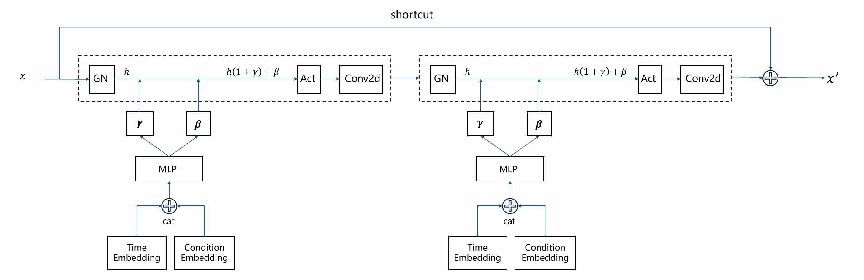
This design enables it to balance stability and controllability.

• Stability: GN prevents variance drift under small batches.

• Control: AdaGN injects noise-level and semantic awareness at every block.

The following figure shows how to inject conditional signal using AdaGN in an UNET residual block.

3.2.2 The Signal Pathways: Skip Connections and Residual Innovations

With a control system in place, the focus shifts to the structural integrity of the network’s information pathways.

• Residual Scaling:

3.1 Architectural Philosophies: U-Net vs. DiT

Normalization has been one of the most fundamental tools in deep learning. Initially, its role was purely that of a stabilizer: preventing exploding/vanishing gradients, reducing internal covariate shift, and enabling deeper networks to converge. However, in diffusion models normalization has undergone a conceptual shift. It is no longer only a numerical safeguard but has become the primary controller for injecting conditioning information such as timesteps, noise scales, class labels, or multimodal embeddings.

3.1.1 Classical Normalization Techniques in Deep Learning

In the architecture of deep neural networks, normalization layers have traditionally served a single, critical purpose: to stabilize training. By re-centering and re-scaling feature distributions, techniques like Batch Normalization and Layer Normalization combat internal covariate shift, ensuring that gradients flow smoothly and training converges reliably. In this role, they act as passive “stabilizers.” All of these methods share the same mathematical template:

where the difference lies in how $\mu$ and $\sigma^2$ are computed (batch, channel, group, or instance scope). At this stage, $\gamma$ and $\beta$ were static learnable parameters. Normalization was a passive stabilizer.

• Batch Normalization (BN) ¹¹: normalizes per channel across the batch and spatial dimensions. Highly effective in CNNs trained with large batches (e.g., ResNet on ImageNet).

  \[\hat{x}_{n,c,h,w} = \frac{x_{n,c,h,w} - \mu_c}{\sqrt{\sigma_c^2 + \epsilon}}\]

  where:

  \[\mu_c = \frac{1}{N \cdot H \cdot W} \sum_{n=1}^N \sum_{h=1}^H \sum_{w=1}^W x_{n,c,h,w}, \quad \sigma_c^2 = \frac{1}{N \cdot H \cdot W} \sum (x_{n,c,h,w} - \mu_c)^2\]

• Layer Normalization (LN) ¹³: normalizes per sample across all channels, making it batch-size independent and ideal for sequence models (Transformers, RNNs).

  \[\hat{x}_{n,c,h,w} = \frac{x_{n,c,h,w} - \mu_n}{\sqrt{\sigma_n^2 + \epsilon}}\]

  where:

  \[\mu_n = \frac{1}{C \cdot H \cdot W} \sum_{c=1}^C \sum_{h=1}^H \sum_{w=1}^W x_{n,c,h,w}, \quad \sigma_n^2 = \frac{1}{C \cdot H \cdot W} \sum (x_{n,c,h,w} - \mu_n)^2\]

• Instance Normalization (IN) ¹⁴: normalizes per sample per channel, used widely in style transfer and image generation for its per-instance invariance.

  \[\hat{x}_{n,c,h,w} = \frac{x_{n,c,h,w} - \mu_{n,c}}{\sqrt{\sigma_{n,c}^2 + \epsilon}}\]

  where:

  \[\mu_{n,c} = \frac{1}{H \cdot W} \sum_{h=1}^H \sum_{w=1}^W x_{n,c,h,w}, \quad \sigma_{n,c}^2 = \frac{1}{H \cdot W} \sum (x_{n,c,h,w} - \mu_{n,c})^2\]

• Group Normalization (GN) ¹²: divides channels into groups and normalizes within each group. Stable under small batch sizes and well-suited to high-resolution CNNs. Divide $C$ channels into $G$ groups. For group $g$:

  \[\hat{x}_{n,c,h,w} = \frac{x_{n,c,h,w} - \mu_{n,g}}{\sqrt{\sigma_{n,g}^2 + \epsilon}}, \quad c \in g\]

  where:

  \[\begin{align} & \mu_{n,g} = \frac{1}{(C/G) \cdot H \cdot W} \sum_{c \in g} \sum_{h=1}^H \sum_{w=1}^W x_{n,c,h,w}, \\[10pt] & \sigma_{n,g}^2 = \frac{1}{(C/G) \cdot H \cdot W} \sum_{c \in g} \sum_{h=1}^H \sum_{w=1}^W (x_{n,c,h,w} - \mu_{n,g})^2 \end{align}\]

3.1.2 From Stabilizer to Controller: Why Normalization Became the Injection Point

Diffusion models forced normalization to evolve. Unlike discriminative models, the denoising network operates under extreme noise regimes, from nearly clean signals to pure Gaussian noise. This requires the model to adapt its feature statistics dynamically depending on the timestep, noise level, or conditioning prompt. Normalization layers became the natural site for this adaptation because:

• Ubiquity: every residual block already contains a normalization step, so conditioning can permeate the entire network.

• Direct statistical control: all of the normalization schemes rely on the learnable affine parameters, the scale ($\gamma$) and shift ($\beta$), to restore feature representation flexibility. These parameters provided a perfect, pre-existing interface for control. By replacing $\gamma$ and $\beta$ with dynamic functions of the conditional vectors, the normalization layer could be “hijacked” to modulate the characteristics of every feature map.

• Lightweight but global influence: a small MLP projecting a condition vector can control feature distributions across all layers without altering the convolutional or attention weights directly.

Thus, normalization transitioned into a controller: not just stabilizing activations, but embedding semantic and structural conditions into the very statistics of feature maps.

3.1.3 U-Net Architectures: GroupNorm and AdaGN

3.1.4 The Transformer Paradigm: DiT, Gating, and AdaLN-Zero

Transformers operate on a fundamentally different data structure: a sequence of tokens of shape $(N, S, D)$, Here, the entire $D$-dimensional vector represents the complete set of features for a single token. This makes Layer Normalization (LayerNorm) ¹³ the ideal choice, as it normalizes across the $D$-dimensional embedding for each token independently.

Consequently, Diffusion Transformers (DiT) ⁹ employ Adaptive Layer Normalization (AdaLN). The principle is identical to AdaGN, but LayerNorm replaces GroupNorm. While the concept has roots in models like StyleGAN2 ¹⁵, its application in Transformers for diffusion was popularized by DiT.

Gate parameter. Many implementations augment AdaLN with a learnable gate $g$, gating provides a way to dynamically control information flow. The most impactful application has been within the MLP layers, through Gated Linear Units (GLU) and its variants. The SwiGLU variant, proposed by Shazeer (2020) ¹⁶, was shown to significantly improve performance by introducing a data-driven, multiplicative gate that selectively passes information through the feed-forward network.

• $g$ is often initialized near 0, ensuring that the residual branch is “silent” at initialization.
• During training, $g$ learns how strongly conditioning should influence the layer.
• This mechanism stabilizes optimization and allows gra

The following figure shows how to inject conditional signal using AdaLN in a transformer block.

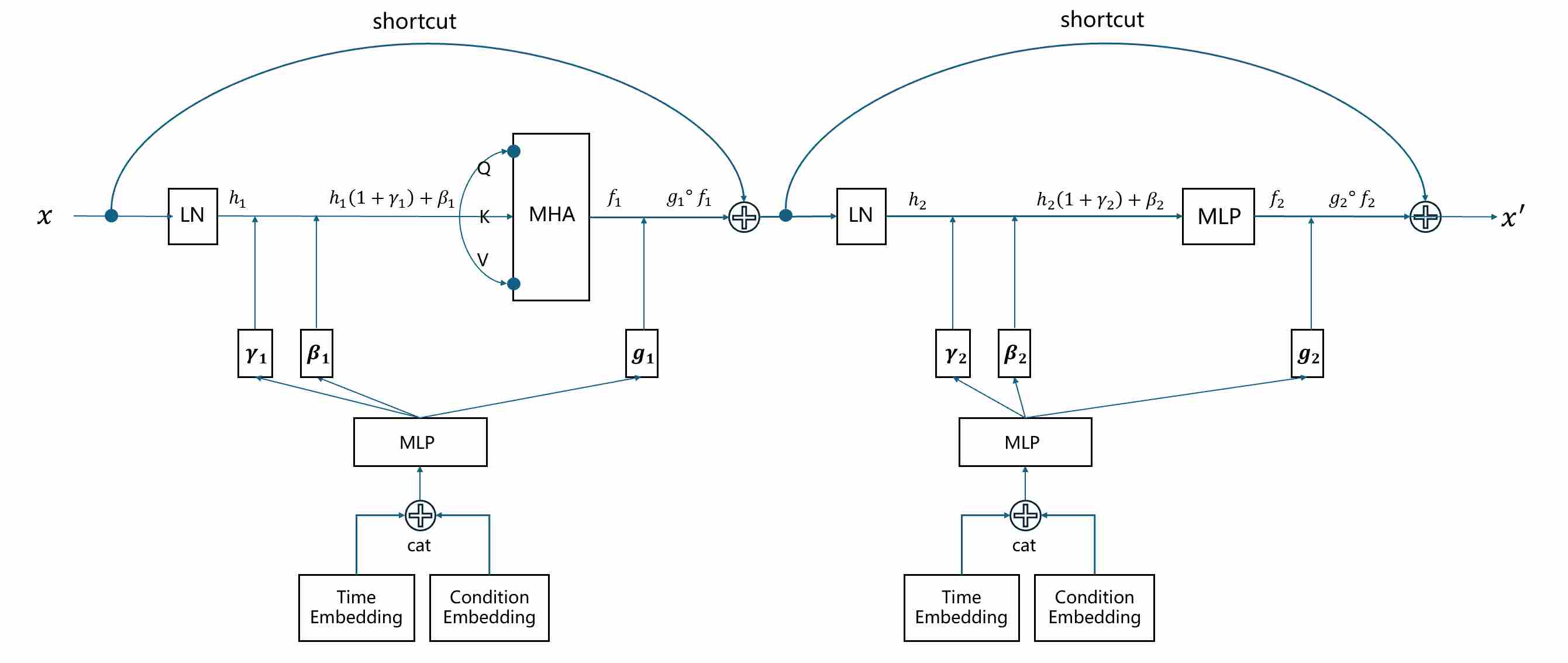
Finally, to solve the unique stability challenges of training extremely deep Transformers, the AdaLN-Zero strategy was introduced in DiT. This is an initialization trick that also functions as a form of gating—a “master switch” that gates the entire residual branch to zero at the start of training. The mechanism is as follows:

• The AdaLN parameters $\gamma$ and $\beta$ are initialized to produce an identity transformation.
• Crucially, the output projection of each attention block and the second linear layer of each MLP block are initialized with all-zero weights.

This ensures that at the start of training, every residual block initially computes the identity function. This creates a pristine “skip-path” for gradients, ensuring stable convergence from the outset. As training progresses, the network learns non-zero weights, gradually “opening the gate” to the residual connections. AdaLN-Zero, combined with the power of gated MLPs and adaptive normalization, provides the trifecta of control and stability needed to scale Transformers to billions of parameters for diffusion models.

9. References