
Diffusion Architectures Part I: Stability-Oriented Designs
📅 Published: | 🔄 Updated:
📘 TABLE OF CONTENTS
- Part I — Foundation and Preliminary
- Part II — Stabilization in U-Net Architectures
- Part III — Stabilization in DiT Architectures
- Part IV — Conclusion
- Part V — References
In our previous article, we examined how diffusion training stability can be improved from the perspective of loss functions and optimization strategies. Yet, stability is not only a matter of training schedules or objectives — the network architecture itself plays a decisive role in determining whether gradients vanish, explode, or propagate smoothly across noise levels.
In this article, we turn to the architectural dimension of stability, comparing U-Net and Transformer-based (DiT) backbones. We highlight how residual pathways, skip connections, and normalization schemes can either stabilize or destabilize training, and present design principles that have proven essential for scaling diffusion models to billions of parameters. Understanding these stability-oriented architectural choices is critical for both researchers aiming to push model robustness and practitioners deploying diffusion systems in real-world settings.
Part I — Foundation and Preliminary
Part I sets up the stability lens we will use throughout this article. Section 1 frames diffusion training stability as a gradient propagation problem across drastically different SNR regimes, highlighting why architectural choices (residual paths, normalization, and skip routes) can decide whether optimization converges or collapses. Section 2 then traces the evolution of diffusion backbones—from classical pixel-space U-Nets, to ADM-era conditioning and scaling refinements, to latent diffusion systems (Stable Diffusion / SDXL), and finally to Transformer-native and hybrid designs—emphasizing how each stage trades inductive bias, capacity, efficiency, and conditioning interfaces. Section 3 distills these developments into a macro-topology contrast between U-Nets and DiTs, clarifying where the stability pressure points live (skip-path regulation vs. per-block numerical stability). This foundation motivates why the remainder of the article splits into backbone-specific stabilization principles.
1. Why Architecture Matters for Stability
Network architecture is more than a vessel for function approximation in diffusion models — it is the key component that determines whether training succeeds or fails.
1.1 Gradient Flow, Conditioning, and Stability
The central difficulty of diffusion training lies in its objective: a single network must operate effectively under wildly different conditions. At each training step, the model is fed an input $x_t$ with a different signal-to-noise ratio. This creates a dual-front war for gradient stability:
At low-noise levels: The input is almost a clean image. The network’s task is subtle refinement. Here, the risk is gradient explosion. A small error in the network’s output can lead to a massive loss gradient, as the model is penalized heavily for deviating even slightly from the ground truth. An unstable architecture will amplify these gradients, causing divergent training steps.
At high-noise levels: The input is nearly pure Gaussian noise. The network’s task is to perceive the faintest hint of structure and begin the process of hallucination. Here, the risk is gradient vanishing. The underlying signal is so weak that gradients can easily diminish to zero as they propagate through a deep network, effectively halting learning for these crucial early stages of generation.
An effective diffusion architecture must therefore act as a precision instrument, maintaining well-behaved gradients across this entire spectrum. This is where architectural choices like residual scaling, normalization layers, and skip connections become critical. They are not just performance-enhancing modules; they are the fundamental regulators of gradient flow, ensuring the network is neither too aggressive at low noise levels nor too passive at high ones.
1.2 Balancing Capacity vs. Robustness
A second challenge lies in the tension between capacity (the ability of the architecture to represent complex distributions) and robustness (the ability to generalize under noisy, unstable conditions).
- Early U-Net designs offered robustness through simplicity and skip connections, but limited capacity for scaling.
- Transformer-based diffusion models (DiT, MMDiT-X) introduced massive representational power, but at the cost of more fragile training dynamics.
- Newer architectures explore hybrid or modular designs — combining convolutional inductive biases, residual pathways, and attention — to find a stable equilibrium between these two competing goals.
1.3 Architecture–Noise Schedule Coupling
Finally, the stability of diffusion training cannot be isolated from the noise schedule. Architectural design interacts tightly with how noise levels are distributed and parameterized:
- A model with time-dependent normalization layers may remain stable under variance-preserving schedules but collapse under variance-exploding ones.
- EDM (Elucidated Diffusion Models) highlight that architecture and preconditioning must be co-designed with the training noise distribution, rather than treated as independent modules.
This coupling implies that progress in diffusion training stability comes not only from better solvers or schedules, but from holistic architectural design that accounts for gradient dynamics, representation capacity, and their interplay with noise parameterization.
2. Evolution of Diffusion Architectures
The architectural journey of diffusion models mirrors the evolution of deep learning itself: from simple convolutional backbones to large-scale Transformers, and now toward specialized multi-modal and efficiency-driven designs. Each stage has sought to reconcile two opposing pressures — increasing representational power while preserving training stability. In this section, we trace this trajectory across six key phases.
2.1 Classical U-Net Foundations
The U-Net architecture 1 is the canonical backbone of early diffusion models such as DDPM 2. Although originally proposed for biomedical image segmentation 1 , its encoder–decoder structure with skip connections turned out to be perfectly suited for denoising across different noise levels. The elegance of U-Net lies not only in its symmetry, but also in how it balances global context extraction with local detail preservation. A typical unet structure applied to the training of diffusion models is as shown below.
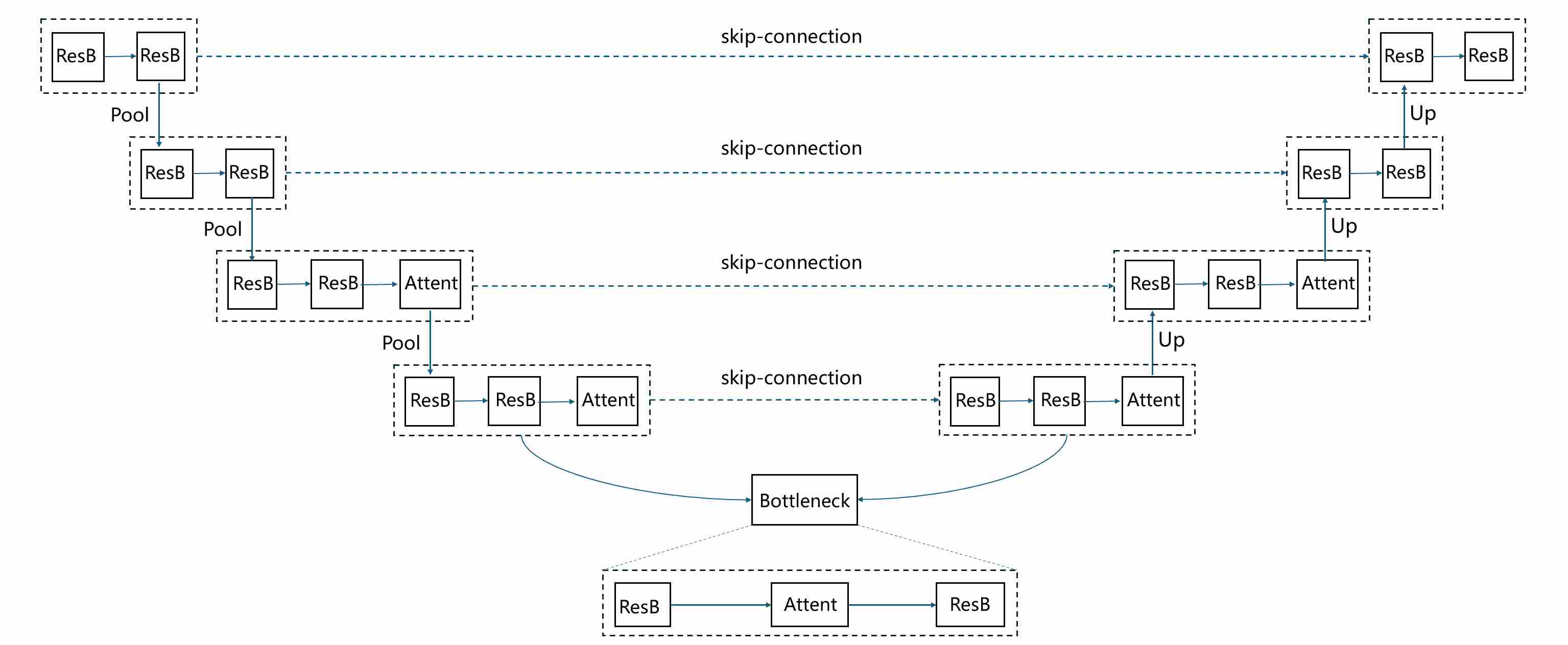
where ResB is a residual block that consists of multiple “norm-act-conv2d” layers. Attent is a self-Attention block.
2.1.1 Encoder: From Local Features to Global Context
The encoder path consists of repeated convolutional residual blocks and downsampling operations (e.g., strided convolutions or pooling). As the spatial resolution decreases and channel width expands, the network progressively shifts its representational emphasis:
- High-resolution feature maps (early layers) capture fine-grained local structures — edges, textures, and small patterns that are critical when denoising images at low noise levels.
- Low-resolution feature maps (deeper layers) aggregate global context — object shapes, spatial layout, and long-range dependencies. This is especially important at high noise levels, when much of the local structure has been destroyed and only global semantic cues can guide reconstruction.
Thus, the encoder effectively builds a multi-scale hierarchy of representations, transitioning from local to global as resolution decreases.
2.1.2 Bottleneck: Abstract Representation
At the center lies the bottleneck block, where feature maps have the smallest spatial size but the largest channel capacity. This stage acts as the semantic aggregator:
- It condenses the global context extracted from the encoder.
- It often includes attention layers (in later refinements) to explicitly model long-range interactions. In the classical U-Net used by DDPM, the bottleneck is still purely convolutional, yet it already plays the role of a semantic “bridge” between encoding and decoding.
2.1.3 Decoder: Reconstructing Local Detail under Global Guidance
The decoder path mirrors the encoder, consisting of upsampling operations followed by convolutional residual blocks. The role of the decoder is not merely to increase resolution, but to inject global semantic context back into high-resolution predictions:
- Upsampling layers expand the spatial resolution but initially lack fine detail.
- Skip connections from the encoder reintroduce high-frequency local features (edges, boundaries, textures) that would otherwise be lost in downsampling.
- By concatenating or adding these skip features to the decoder inputs, the network fuses global context (from low-res encoder features) with local precision (from high-res encoder features).
This synergy ensures that the denoised outputs are both semantically coherent and visually sharp.
2.1.4 Timestep Embedding and Conditioning
Unlike the U-Net’s original role in segmentation, a diffusion U-Net must also be conditioned on the diffusion timestep $t$, since the network’s task changes continuously as noise levels vary. In the classical DDPM implementation, this conditioning is realized in a relatively simple but effective way:
Sinusoidal embedding. Each integer timestep $t$ is mapped to a high-dimensional vector using sinusoidal position encodings (analogous to Transformers), ensuring that different timesteps are represented as distinct, smoothly varying signals.
MLP transformation. The sinusoidal embedding is passed through a small multilayer perceptron (usually two linear layers with a SiLU activation) to produce a richer time embedding vector $\mathbf{z}_t$.
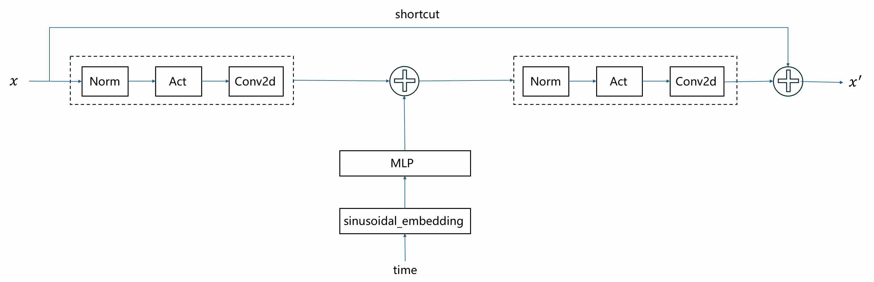
Additive injection into residual blocks. In every residual block of the U-Net, $\mathbf{z}_t$ is projected to match the number of feature channels and then added as a bias term to the intermediate activations (typically after the first convolution).
This additive conditioning allows each residual block to adapt its computation based on the current noise level, without introducing extra normalization or complex modulation. The following figure shows the way how to inject timestep $t$ in each residual block.
However, additive injection suffers from several inherent limitations, making it rarely used in modern state-of-the-art models. By simply adding conditional embeddings to the intermediate features, it only provides a uniform shift across all dimensions, which restricts its expressiveness. This coarse modulation often leads to an information bottleneck, as rich and structured conditions (e.g., long text prompts or spatial guidance) cannot be aligned effectively with image features. Moreover, additive injection lacks adaptability to the varying statistics across different layers of the network, which can cause instability during training and suboptimal conditioning performance. We will discuss more complicated injected strategies in section 4.1 and section 5.1
2.1.5 Why U-Net Works Well for Diffusion
In diffusion training, inputs vary drastically in signal-to-noise ratio:
- At low noise levels, local details still survive; skip connections ensure these details propagate to the output.
- At high noise levels, local detail is destroyed; the decoder relies more on global semantics from the bottleneck.
- Across all levels, the encoder–decoder interaction guarantees that both local fidelity and global plausibility are preserved.
This explains why U-Nets became the default backbone: their multi-scale design matches perfectly with the multi-scale nature of noise in diffusion models. Later improvements (attention layers, latent-space U-Nets, Transformer backbones) all build upon this foundation, but the core idea remains: stability in diffusion training emerges from balanced local–global feature fusion.
2.2 ADM Improvements (Ablated Diffusion Models)
While the classical U-Net backbone of DDPM demonstrated the feasibility of diffusion-based generation, it was still limited in stability and scalability. In the landmark work “Diffusion Models Beat GANs on Image Synthesis” 3, the authors performed extensive ablations to identify which architectural and training choices were critical at ImageNet scale. The resulting recipe is commonly referred to as ADM (Ablated Diffusion Models). Rather than introducing a single new module, ADM represents a carefully engineered upgrade to the baseline U-Net, designed to balance capacity, conditioning, and stability.
2.2.1 Scaling the U-Net: Wider Channels and Deeper Residual Blocks
The most straightforward but highly effective change was scaling up the model. The ADM UNet is significantly larger than the one used in the original DDPM paper.
- Wider Channels: The base channel count was increased (e.g., from 128 to 256), and the channel multipliers for deeper layers were adjusted, resulting in a much wider network.
- More Residual Blocks: The number of residual blocks per resolution level was increased, making the network deeper.
Why it helps: A larger model capacity allows the network to learn more complex and subtle details of the data distribution, leading to a direct improvement in sample fidelity.
2.2.2 Multi-Resolution Self-Attention
While DDPM’s UNet used self-attention, it was typically applied only at a single, low resolution (e.g., 16x16). ADM recognized that long-range dependencies are important at various scales.
In ADM, Self-attention blocks were added at multiple resolutions (e.g., 32x32, 16x16, and 8x8). Additionally, the number of attention heads was increased.
- Attention at higher resolutions (32x32) helps capture relationships between medium-sized features and textures;
- Attention at lower resolutions (8x8) helps coordinate the global structure and semantic layout of the image.
Why it helps: This multi-scale approach gives the model a more holistic understanding of the image, preventing structural inconsistencies and improving overall coherence.
2.2.3 Conditioning via Adaptive Group Normalization (AdaGN)
This is arguably the most significant architectural contribution of ADM. It fundamentally changes how conditional information (like timesteps and class labels) is integrated into the network.
In DDPM: The time embedding was processed by an MLP and then simply added to the feature maps within each residual block. This acts as a global bias, which is a relatively weak form of conditioning.
In ADM (AdaGN) 4: The model learns to modulate the activations using the conditional information. The process is as follows: a). The timestep embedding and the class embedding (for class-conditional models) are combined into a single conditioning vector; b). This vector is passed through a linear layer to predict two new vectors: a scale ($\gamma$) and a shift ($\beta$) parameter for each channel. c). Within each residual block, the feature map undergoes Group Normalization, and then its output is modulated by these predicted parameters.
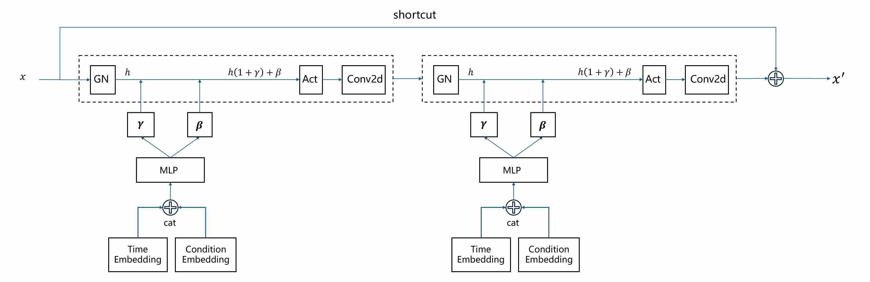
Why it helps: Modulation is a much more powerful mechanism than addition. It allows the conditional information to control the mean and variance of each feature map on a channel-by-channel basis. This gives the model fine-grained control over the generated features, dramatically improving its ability to adhere to the given conditions (i.e., generating a specific class at a specific noise level).
2.2.4 BigGAN-inspired Residual Blocks for Up/Downsampling
ADM also identifies that the choice of downsampling and upsampling operations affects stability.
In DDPM: Downsampling might be a simple pooling (max pooling or mean pooling) or strided convolution, and upsampling might be a standard upsample layer followed by a convolution.
In ADM: The upsampling and downsampling operations were integrated into specialized residual blocks (as shown below), a design inspired by the highly successful BigGAN architecture 5. This ensures that information flows more smoothly as the resolution changes, minimizing information loss.
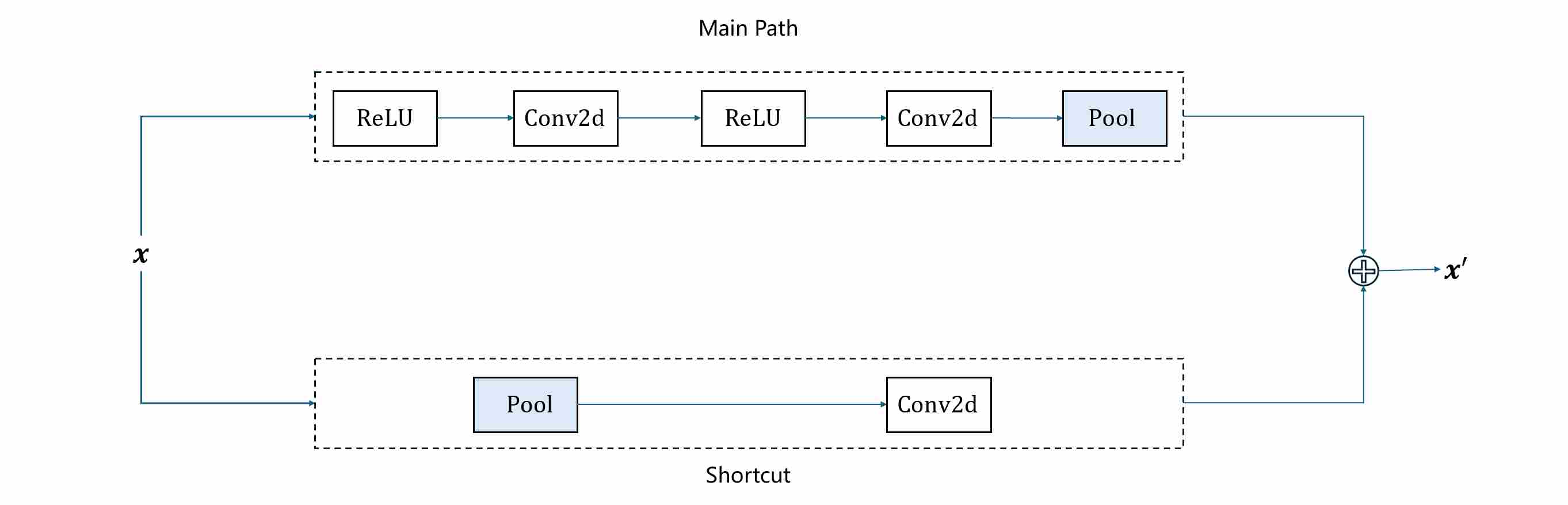
It favors strided convolutions for downsampling and nearest-neighbor upsampling followed by convolution for upsampling.
Why it helps: This leads to better preservation of features across different scales, contributing to sharper and more detailed final outputs.
2.2.5 Rescaling of Residual Connections
For very deep networks, it’s crucial to maintain well-behaved activations. ADM introduced a simple but effective trick: The output of each residual block was scaled by a constant factor of 1/${\sqrt{2}}$ before being added back to the skip connection.
Why it helps: This technique helps to balance the variance contribution from the skip connection and the residual branch, preventing the signal from exploding in magnitude as it passes through many layers. This improves training stability for very deep models.
2.2.6 Why ADM Matters for Stability
Relative to the classical DDPM U-Net, in conclusion, the ADM UNet is a masterclass in architectural refinement. By systematically enhancing every major component—from its overall scale to the precise mechanism of conditional injection—it provided the powerful backbone necessary for diffusion models to finally surpass GANs in image synthesis quality.
2.3 Latent U-Net: The Efficiency Revolution with Stable Diffusion
While the ADM architecture (Section 2.2) marked the pinnacle of pixel-space diffusion models, achieving state-of-the-art quality by meticulously refining the U-Net, it faced a significant and inherent limitation: computational cost. Training and running diffusion models directly on high-resolution images (e.g., 512x512 or 1024x1024) is incredibly demanding in terms of both memory and processing power. The U-Net must process massive tensors at every denoising step, making the process slow and resource-intensive.
The introduction of Latent Diffusion Models (LDMs) 6, famously realized in Stable Diffusion, proposed a revolutionary solution: instead of performing the expensive diffusion process in the high-dimensional pixel space, why not perform it in a much smaller, perceptually equivalent latent space? This insight effectively decouples the task of perceptual compression from the generative learning process, leading to a massive leap in efficiency and accessibility.
2.3.1 The Core Idea: Diffusion in a Compressed Latent Space
The training architecture of LDM is a two-stage process.
Stage 1: Perceptual Compression. A powerful, pretrained Variational Autoencoder (VAE) is trained to map high-resolution images into a compact latent representation and back. The encoder, $E$, compresses an image x into a latent vector $z = E(x)$. The decoder, $D$, reconstructs the image from the latent, \(\tilde x = D(z)\). Crucially, this is not just any compression; it is perceptual compression, meaning the VAE is trained to discard high-frequency details that are imperceptible to the human eye while preserving critical semantic and structural information.
Stage 2: Latent Space Diffusion. Instead of training a U-Net on images x, we train it on the latent codes $z$. The forward diffusion process adds noise to $z$ to get $z_t$, and the U-Net’s task is to predict the noise in this latent space.
The impact of this shift is dramatic. A 512x512x3 pixel image (786,432 dimensions) can be compressed by the VAE into a 64x64x4 latent tensor (16,384 dimensions)—a 48x reduction in dimensionality. The U-Net now operates on these much smaller tensors, enabling faster training and significantly lower inference requirements.
The full generative (inference) process for a text-to-image model like Stable Diffusion is as follows:
- Stage 1: Text Prompt $\to$ Text Encoder $\to$ Conditioning Vector $c$.
- Stage 2: Random Noise $z_T$ $\to$ U-Net Denoising Loop in Latent Space, conditioned on $c$ $\to$ Clean Latent \(z_0\).
- Stage 3: Clean Latent $z_0$ $\to$ VAE Decoder $\to$ Final Image $x$.
2.3.2 Architectural Breakdown of the Latent U-Net
While the Latent U-Net, exemplified by Stable Diffusion, inherits its foundational structure from the ADM architecture (i.e., a U-Net with residual blocks and multi-resolution self-attention), it introduces several profound modifications. These are not mere tweaks but fundamental redesigns necessary to operate efficiently in a latent space and to handle the sophisticated conditioning required for text-to-image synthesis.
A. Conditioning Paradigm Shift: From AdaGN to Cross-Attention
This is the most critical evolution from the ADM architecture. ADM perfected conditioning for global, categorical information (like a single class label), whereas Stable Diffusion required a mechanism for sequential, localized, and compositional information (a text prompt).
ADM’s Approach (Global Conditioning): ADM injected conditions (time embedding, class embedding) via adaptive normalization (AdaGN/FiLM): A single class embedding vector is combined with the time embedding. This unified vector is then projected to predict scale and shift parameters that modulate the entire feature map within a ResBlock.
Limitation: This is an “all-at-once” conditioning signal. The network knows it needs to generate a “cat,” and this instruction is applied globally across all spatial locations. It cannot easily handle a prompt like “a cat sitting on a chair,” because the conditioning signal for “cat” and “chair” cannot be spatially disentangled.
Latent U-Net’s Approach (Localized Conditioning): Latent U-Nets instead integrate text tokens (from a frozen text encoder, e.g., CLIP) using cross-attention at many/most resolutions: Instead of modulating activations, the U-Net directly incorporates the text prompt’s token embeddings at multiple layers. A text encoder (e.g., CLIP) first converts the prompt “a cat on a chair” into a sequence of token embeddings: [
, a, cat, on, a, chair, ]. These embeddings form the Key (K) and Value (V) for the cross-attention mechanism. The U-Net’s spatial features act as the Query (Q). At each location in the feature map, the Query can “look at” the sequence of text tokens and decide which ones are most relevant. A region of the feature map destined to become the cat will learn to place high attention scores on the “cat” token, while a region for the chair will attend to the “chair” token.
\[\begin{aligned} \small & \text{Attn}(Q,\,K,\,V)=\text{softmax}(QK^T/\sqrt{d})V,\quad \\[10pt] & Q=\text{latent features},\quad K,V=\text{text tokens} \end{aligned}\]
B. Self-Attention vs. Cross-Attention
The modern Latent U-Net block now has a clear and elegant division of labor: Self-Attention and Cross-Attention. This dual-attention design is profoundly more powerful than ADM’s global conditioning, enabling the complex compositional generation we see in modern text-to-image models. Cross-Attention usually at multiple scales, often after each residual block.
Self-Attention: capture long-range dependencies and ensure global structural/semantic consistency. Convolutions and skip connections excel at local detail, but struggle to enforce coherence across distant regions. Self-attention fills this gap. Self-Attention typically only at low-resolution stages (e.g., 16×16 or 8×8).
Cross-Attention: enable multimodal alignment, projecting language semantics onto spatial locations. Coarse-scale cross-attn controls global layout, style, and subject placement. Fine-scale cross-attn refines local textures, materials, and fine details.
C. Adapting the Training Objective for Latent Space: $v$-prediction
Another key adaptation that makes training deep and powerful U-Nets in latent space more robust and effective is the choice of objective.
We have discussed four common prediction targets to train diffusion models (post). Through analysis and comparison, we found that $v$-prediction has the best stability, this led LDM to shift towards using $v$ instead of $\epsilon$ to achieve more stable training results.
D. Perceptual Weighting in Latent Space
In Latent Diffusion Models, diffusion is not trained directly in pixel space but in the latent space of a perceptual autoencoder (a VAE). The latent representation is much smaller (e.g., 64×64×4 for a 512×512 image) and is designed to preserve perceptually relevant information.
However, if we train the diffusion model with a plain mean squared error (MSE) loss on the latent vectors, you implicitly treat all latent dimensions and spatial positions as equally important. In practice:
- Some latent channels carry critical perceptual information (edges, textures, semantics).
- Other channels encode redundant or imperceptible details.
Without adjustment, the diffusion model may spend too much gradient budget on parts of the latent space that have little impact on perceptual quality. Perceptual weighting introduces a weighting factor $w(z)$ into the diffusion loss, so that errors in perceptually important latent components are emphasized:
\[\mathcal{L} = \mathbb{E}_{z,t,\epsilon}\big[\, w(z)\,\|\epsilon - \epsilon_\theta(z_t, t)\|^2 \,\big],\]There are different ways to define $w(z)$:
Channel-based weighting from the VAE
- Estimate how much each latent channel contributes to perceptual fidelity (e.g., by measuring sensitivity of the VAE decoder to perturbations in that channel).
- Assign larger weights to channels that strongly affect the decoded image.
Feature-based weighting (perceptual features)
- Decode the latent $z$ back to image space $x=D(z)$.
- Extract perceptual features $\phi(x)$ (e.g., from a VGG network or LPIPS).
- Estimate how sensitive these features are to changes in $z$. Latent dimensions with high sensitivity get higher weights.
Static vs. adaptive weighting
- Static: Precompute a set of per-channel weights (averaged over the dataset).
- Adaptive: Compute weights on the fly per sample or per timestep using Jacobian-vector product tricks.
In summary:
- Focus on perceptual quality: Gradients are concentrated on latent components that most affect the decoded image quality.
- Suppress irrelevant gradients: Channels that mostly encode imperceptible high-frequency noise are downweighted.
- More stable training: The denoiser learns where its predictions matter most, reducing wasted updates and improving convergence.
2.3.3 Evolution to SDXL: Refining the Latent U-Net Formula
While Stable Diffusion models 1.x and 2.x established the power of the Latent Diffusion paradigm, Stable Diffusion XL (SDXL) 7 represents a significant architectural leap forward. It is not merely a larger model but a systematically re-engineered system designed to address the core limitations of its predecessors, including native resolution, prompt adherence, and aesthetic quality. The following sections provide a detailed technical breakdown of the key architectural innovations in SDXL.
A. Two-Stage Cascade Pipeline: The Base and Refiner Models
To achieve the highest level of detail and aesthetic polish, SDXL introduces an optional but highly effective two-stage generative process, employing two distinct models.
The Core Problem: The Global and Local Dilemma. A single diffusion model faces a challenging balancing act. During the denoising process, it must simultaneously:
- Establish Global Coherence: Correctly interpret the prompt to create a plausible composition, with proper object placement, anatomy, lighting, and color harmony. This is a low-frequency task.
- Render Fine Details: Generate intricate, high-frequency textures like skin pores, fabric weaves, hair strands, and sharp edges. This is a high-frequency task.
Stage 1: The Base Model. The base model is the workhorse of the pipeline. Its primary responsibility is to create a structurally sound and semantically correct foundation for the image.
- Function: It performs the bulk of the denoising process, starting from pure Gaussian noise ($z_T$) and running for a majority of the sampling steps (e.g., from step 1000 down to step 200). It is tasked with the “heavy lifting” of interpreting the prompt and translating it into a coherent visual scene.
- Strengths: The base model, being very large and powerful (e.g., the 2.6 billion parameter U-Net in SDXL), excels at:
- Composition and Layout: Arranging objects in the scene according to the prompt.
- Color and Lighting: Establishing a consistent and harmonious color palette and lighting scheme.
- Semantic Accuracy: Ensuring subjects and concepts from the prompt are correctly represented and interact plausibly.
- Output: It produces a latent representation that is structurally complete and visually strong. You can think of its output as a high-quality, fully-formed painting that is conceptually finished but could still benefit from a final layer of polish and fine-tuning.
Stage 2: The Refiner Model. The refiner model takes over where the base model leaves off. It is not a general-purpose generator; it is a specialist trained for a very specific task: adding the final touch of realism and quality.
- Function: It takes the latent output from the base model as its starting point. This is crucial—it does not start from pure noise. It starts from a latent that is already in a low-noise state. It then performs a small number of final denoising steps (e.g., from step 200 down to 0).
- Specialized Training: This is its secret weapon. The refiner is trained exclusively on images with a low level of noise. This makes it an “expert” at high-fidelity rendering. It doesn’t need to know how to create a face from chaos, but it is exceptionally good at taking an almost-perfect face and adding realistic skin texture, subtle reflections in the eyes, and individual hair strands.
- Strengths: The refiner focuses solely on: High-Frequency Detail Injection: sharpening edges, clarifying text, and adding intricate textures; Artifact Correction: Smoothing out minor imperfections or noise left over by the base model; Aesthetic Enhancement: Applying a final “polish” that pushes the image towards a higher level of photorealism or artistic finish.
Impact: This ensemble-of-experts approach allows for a division of labor. The base model ensures robust composition, while the refiner specializes in aesthetic finalization. The result is an image that benefits from both global coherence and local, high-frequency richness, achieving a level of quality that is difficult for a single model to produce consistently.
B. Substantially Larger and More Robust U-Net Backbone
The most apparent upgrade in SDXL is its massively scaled-up U-Net, which serves as the core of the base model. This expansion goes beyond a simple increase in parameter count to include strategic design choices.
Increased Capacity: The SDXL base U-Net contains approximately 2.6 billion parameters, a nearly threefold increase compared to the ~860 million parameters of the U-Net in SD 1.5. This additional capacity is crucial for learning the more complex and subtle features required for high-resolution 1024x1024 native image generation.
Deeper and Wider Architecture: The network’s depth (number of residual blocks) and width (channel count) have been significantly increased. Notably, the channel count is expanded more aggressively in the middle blocks of the U-Net. These blocks operate on lower-resolution feature maps (e.g., 32x32) where high-level semantic information is most concentrated. By allocating more capacity to these semantic-rich stages, the model enhances its ability to reason about object composition and global scene structure, directly mitigating common issues like malformed anatomy (e.g., extra limbs) seen in earlier models at high resolutions.
Refined Attention Mechanisms: The distribution and configuration of the attention blocks (both self-attention and cross-attention) across different resolution levels were re-evaluated and optimized. This ensures a more effective fusion of spatial information (from the image features) and semantic guidance (from the text prompt) at all levels of abstraction.
Impact: This fortified U-Net backbone is the primary reason SDXL can generate coherent, detailed, and aesthetically pleasing images at a native 1024x1024 resolution, a feat that was challenging for previous versions without significant post-processing or specialized techniques.
C. The Dual Text Encoder: A Hybrid Approach to Prompt Understanding
Perhaps the most innovative architectural change in SDXL is its departure from a single text encoder. SDXL employs a dual text encoder strategy to achieve a more nuanced and comprehensive understanding of user prompts.
OpenCLIP ViT-bigG: This is the larger of the two encoders and serves as the primary source of high-level semantic and conceptual understanding. Its substantial size allows it to grasp complex relationships, abstract concepts, and the overall sentiment or artistic intent of a prompt (e.g., “a majestic castle on a hill under a starry night”).
CLIP ViT-L: The second encoder is the standard CLIP model used in previous Stable Diffusion versions. It excels at interpreting more literal, granular, and stylistic details in the prompt, such as specific objects, colors, or artistic styles (e.g., “a red car,” “in the style of Van Gogh”).
Mechanism of Fusion: During inference, the input prompt is processed by both encoders simultaneously. The resulting sequences of token embeddings are then concatenated along the channel dimension before being fed into the U-Net’s cross-attention layers. This combined embedding provides the U-Net with a richer, multi-faceted conditioning signal.
Impact: This hybrid approach allows SDXL to reconcile two often competing demands: conceptual coherence and stylistic specificity. The model can understand the “what” (from ViT-L) and the “how” (from ViT-bigG) of a prompt with greater fidelity, leading to superior prompt adherence and the ability to generate complex, well-composed scenes that match the user’s intent more closely.
D. Micro-Conditioning for Resolution and Cropping Robustness
SDXL introduces a subtle yet powerful form of conditioning that directly addresses a common failure mode in generative models: sensitivity to image aspect ratio and object cropping.
The Problem: Traditional models are often trained on square-cropped images of a fixed size. When asked to generate images with different aspect ratios, they can struggle, often producing unnatural compositions or cropped subjects.
SDXL’s Solution: During training, the model is explicitly conditioned on several metadata parameters in addition to the text prompt:
- original height and original width: The dimensions of the original image before any resizing or cropping.
- crop top and crop left: The coordinates of the top-left corner of the crop.
- target height and target width: The dimensions of the final generated image.
Mechanism of Injection: These scalar values are converted into a fixed-dimensional embedding vector. This vector is then added to the sinusoidal time embedding before being passed through the AdaGN layers of the U-Net’s residual blocks.
Impact: By making the model “aware” of the resolution and framing context, SDXL learns to generate content that is appropriate for the specified canvas. This significantly improves its ability to handle diverse aspect ratios and dramatically reduces instances of unwanted cropping, leading to more robust and predictable compositional outcomes.
2.4 Transformer-based Designs
While latent U-Nets (Section 2.3) significantly improved efficiency and multimodal conditioning, they still retained convolutional inductive biases and hierarchical skip pathways. Due to the success of Transformers 8 in large-scale NLP tasks, the next stage in the evolution of diffusion architectures explores whether Transformers can serve as the primary backbone for diffusion models. This marks a decisive shift from UNET-dominated designs to Transformer-native backbones, most notably exemplified by the Diffusion Transformer (DiT) 9 family and its successors.
2.4.1 Motivation for Transformer Backbones
Convolution-based U-Nets provide strong locality and translation invariance, but they impose rigid inductive biases:
Locality and Global Context: Convolutions capture local patterns well but require deep hierarchies to model long-range dependencies. U-Nets solve this partially through down/upsampling and skip connections, but global coherence still relies on explicit attention layers carefully placed at coarse scales.
Transformers, by contrast, model all-pair interactions directly via attention, making them natural candidates for tasks where global semantics dominate.
Benefit from Scaling laws: Recent work shows that Transformers scale more predictably with dataset and parameter count, whereas CNNs saturate earlier. Diffusion training, often performed at very large scales, benefits from architectures that exhibit similar scaling behavior.
Unified multimodal processing.: Many diffusion models condition on text or other modalities. Transformers provide a token-based interface: both images (as patch embeddings) and text (as word embeddings) can be treated uniformly, simplifying multimodal alignment.
Thus, a Transformer-based backbone promises to simplify design and leverage established scaling laws, potentially achieving higher fidelity with cleaner training dynamics.
2.4.2 Architectural Characteristics of Diffusion Transformers
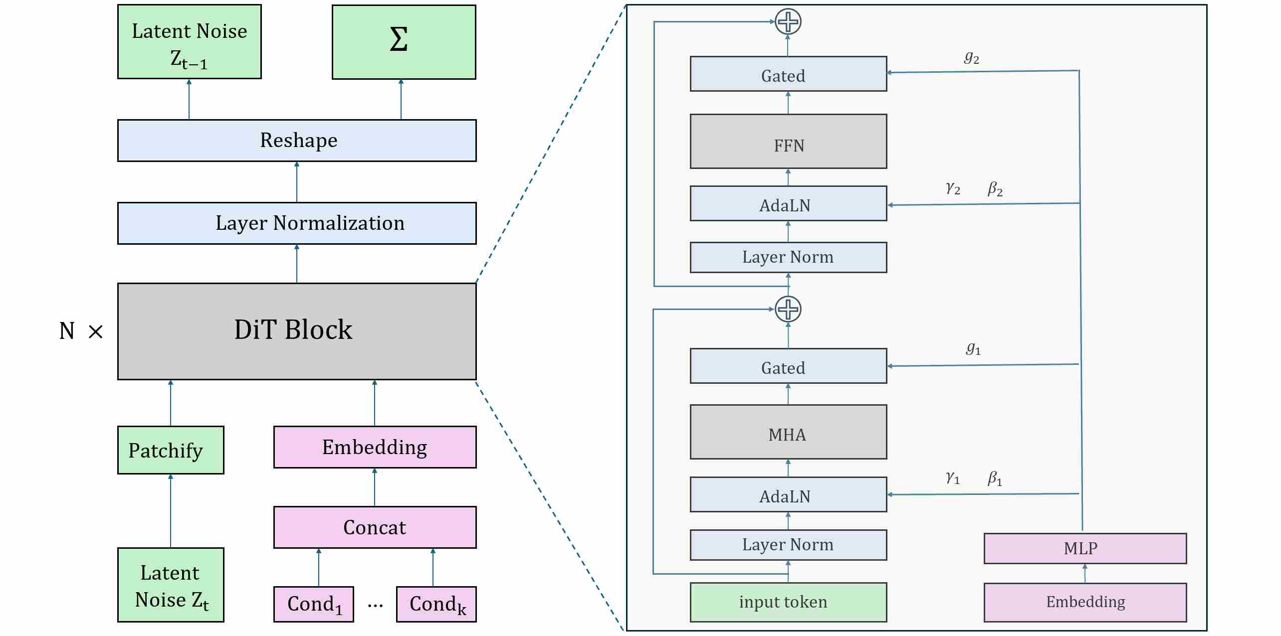
The Diffusion Transformer (DiT) proposed by Peebles & Xie (2022) was the first systematic exploration of replacing U-Nets with ViT-style Transformers for diffusion.
- Patch tokenization: Instead of convolutions producing feature maps, the input (pixels or latents) is divided into patches (e.g., 16×16), each mapped to a token embedding. This yields a sequence of tokens that a Transformer can process natively.
- Class and time conditioning: As in ADM, timestep and class embeddings are injected not by concatenation but by scale-and-shift modulation of normalization parameters. The different is that, instead of AdaGN, DiT uses Adaptive LayerNorm (AdaLN).
- Global self-attention: Unlike U-Nets, where attention is inserted at selected resolutions, DiT-style models apply self-attention at every layer. This uniformity eliminates the need to decide “where” to place global reasoning — it is omnipresent.
- Scalability: Transformers scale more gracefully with depth and width. With large batch training and data-parallelism, models like DiT-XL can be trained efficiently on modern accelerators.
DiT demonstrates that diffusion models do not require convolutional backbones. However, it also reveals that training Transformers for denoising is more fragile: optimization can collapse without careful normalization (AdaLN-Zero) and initialization tricks.
The Diffusion Transformer (DiT) architecture is as shown below.
2.4.3 Hybrid Designs: Marrying U-Net and Transformer Strengths
Pure Transformers are computationally expensive, especially at high resolutions. To balance efficiency and quality, several hybrid architectures emerged:
U-Net with Transformer blocks — many models, including Stable Diffusion v2 and SDXL, interleave attention layers (which are Transformer sub-blocks) into convolutional U-Nets. This compromise preserves locality while still modeling long-range dependencies.
Perceiver-style cross-attention. Conditioning (e.g., text embeddings) can be injected via cross-attention, a Transformer-native mechanism that naturally fuses multimodal tokens.
MMDiT (Multimodal DiT) in Stable Diffusion 3. Here, both image latents and text tokens are treated as tokens in a single joint Transformer sequence. Queries, keys, and values are drawn from both modalities, enabling a fully symmetric text–image fusion mechanism without the asymmetry of U-Net cross-attention layers.
2.5 Extensions to Video and 3D Diffusion
The success of diffusion models on static images naturally prompted their extension to more complex, higher-dimensional data like video and 3D scenes. This required significant architectural innovations to handle the temporal dimension in video and the complex geometric representations of 3D objects, all while maintaining consistency and stability.
2.5.1 Video U-Net: Introducing the Temporal Dimension
The most direct way to adapt an image U-Net for video generation is to augment it with mechanisms for processing the time axis. This gave rise to the Spatio-Temporal U-Net.
A. Temporal Layers for Consistency
A video can be seen as a sequence of image frames, i.e., a tensor of shape $(B, T, C, H, W)$. A standard 2D U-Net processes each frame independently, leading to flickering and temporal incoherence. To solve this, temporal layers are interleaved with the existing spatial layers:
- Temporal Convolutions: 3D convolution layers (e.g., with a kernel size of $(3, 3, 3)$ for $(T, H, W)$) replace or supplement the standard 2D convolutions. This allows features to be aggregated from neighboring frames.
- Temporal Attention: This is the more powerful and common approach. After a spatial self-attention block that operates within each frame, a temporal self-attention block is added. In this block, a token at frame $t$ attends to corresponding tokens at other frames ($t-1$, $t+1$, etc.). This explicitly models long-range motion and appearance consistency across the entire video clip.
Models like Stable Video Diffusion (SVD) build upon a pretrained image LDM and insert these temporal attention layers into its U-Net. By first training on images and then fine-tuning on video data, the model learns temporal dynamics while leveraging the powerful prior of the image model.
B. Conditioning on Motion
To control the dynamics of the generated video, these models are often conditioned on extra information like frames per second (FPS) or motion “bucket” IDs representing the amount of camera or object motion. This conditioning is typically injected alongside the timestep embedding, allowing the model to generate videos with varying levels of activity.
2.5.2 3D Diffusion: Generating Representations Instead of Pixels
Generating 3D assets is even more challenging due to the complexity of 3D representations (meshes, voxels, NeRFs) and the need for multi-view consistency. A breakthrough approach has been to use diffusion models to generate the parameters of a 3D representation itself, rather than rendering pixels directly.
A. Diffusion on 3D Gaussian Splatting Parameters
3D Gaussian Splatting (3D-GS) has emerged as a high-quality, real-time-renderable 3D representation. A scene is represented by a collection of 3D Gaussians, each defined by parameters like position (XYZ), covariance (scale and rotation), color (RGB), and opacity.
Instead of a U-Net that outputs an image, models like 3D-GS Diffusion use an architecture (often a Transformer) to denoise a set of flattened Gaussian parameters. The process works as follows:
- Canonical Representation: A set of initial Gaussian parameters is created (e.g., a sphere or a random cloud).
- Diffusion Process: Noise is added to this set of parameters (position, color, etc.) over time.
- Denoising Network: A Transformer-based model takes the noisy parameter set and the conditioning signal (e.g., text or a single image) and predicts the clean parameters.
- Rendering: Once the denoised set of Gaussian parameters is obtained, it can be rendered from any viewpoint using a differentiable 3D-GS renderer to produce a 2D image.
This approach elegantly separates the generative process (in the abstract parameter space) from the rendering process. By operating on the compact and structured space of Gaussian parameters, the model can ensure 3D consistency by design, avoiding the view-incoherence problems that plague naive image-space 3D generation.
3. Architectural Philosophies: U-Net vs. DiT
Before diving into specific mechanisms, we must first understand the high-level topological differences between U-Nets and DiTs. The very shape of these architectures dictates their inherent strengths, weaknesses, and, consequently, where the primary “pressure points” for stability lie.
3.1 U-Net Macro Topology
We have already covered most of the knowledge about the UNET structure in Section 2, and here we only provide a brief summary. The U-Net family is characterized by its encoder–decoder symmetry with long skip connections that link features at the same spatial resolution.
Strengths: Skip connections preserve fine-grained details lost during downsampling, and they dramatically shorten gradient paths, alleviating vanishing gradients in very deep convolutional stacks.
Weaknesses: The powerful influence of the skip connections can be a double-edged sword. Overly strong skips can dominate the decoder, reducing reliance on deeper semantic representations. They can also destabilize training when the variance of encoder features overwhelms decoder activations.
Implication: For U-Nets, stabilization hinges on how residual and skip pathways are regulated — via normalization, scaling, gating, or progressive fading.
3.2 DiT Macro Topology
Similarily, we have already covered most of the knowledge about the UNET structure in Section 2, and here we only provide a brief summary. Diffusion Transformers (DiT) abandon encoder–decoder symmetry in favor of a flat stack of homogeneous blocks. Every layer processes a sequence of tokens with identical embedding dimensionality.
Strengths: This design is remarkably simple, uniform, and highly scalable. It aligns perfectly with the scaling laws that have driven progress in large language models.
Weaknesses: Without long skips, there are no direct gradient highways. The deep, uninterrupted stack can easily amplify variance or degrade gradients with each successive block. A small numerical error in an early layer can be compounded dozens of times, leading to catastrophic failure. Stability pressure is concentrated entirely on per-block design.
Implication: For DiTs, the central question is how to stabilize each block internally, rather than balancing long-range skips.
3.3 Summary of Divergent
Overall, there are significant differences in the optimization of stability between this two architectures.
U-Net: Stability is equal to manage the interplay between skip connections and residual blocks.
DiT: Stability is equal to ensure each block is numerically stable under deep stacking. This divergence explains why U-Nets emphasize skip/residual design, while DiTs emphasize normalization, residual scaling, and gated residual paths.
Part II — Stabilization in U-Net Architectures
In diffusion / flow-matching U-Nets, the long skip pathway (encoder → decoder at the same resolution) is simultaneously a quality driver and a stability risk. It is a quality driver because it carries high-resolution spatial detail; it is a stability risk because it can become an uncontrolled bypass that injects noise, overwhelms semantic features, and amplifies forward/backward oscillations.
To reason about all skip-connection improvements in a single language, we treat the skip fusion at each decoder stage as a two-stream operator:
\[y=\mathrm{Fuse}\Big(w_d(t,\ell,z)\odot \phi_d(d, z),\;\; w_s(t,\ell,z)\odot \phi_s(s, z),\;\; z\Big),\]The meanings of each symbol are summarized in following table:
| Symbol | Meaning | Variation Dimensions |
|---|---|---|
| $d$ | Decoder feature | Spatial + Channel |
| $s$ | Skip feature (encoder output at the same resolution) | Spatial + Channel |
| $\phi_d, \phi_s$ | Feature transformation functions | Learnable / Fixed |
| $w_d, w_s$ | Weight / Gating / Scaling factors | Timestep / Layer / Condition / Spatial |
| $t$ | Diffusion timestep | $[0, T]$ or $[0, 1]$ |
| $\ell$ | Layer index | Integer |
| $z$ | External conditions | Text / Image / Control signals |
| $\mathrm{Fuse}$ | Fusion operator | Addition / Concatenation / Attention |
4. What Goes Wrong with Naive Skip Connections?
In the classic implementations of DDPM, a typical “plain” U-Net skip can be written as either addition or concat.
\[y = d\;+\;s \quad \text{or} \quad y =\mathrm{Proj}([d;\;s])\]Both are special cases of the unified operator with fixed weights and identity transforms:
\[w_d=w_s=1,\qquad \phi_d=\phi_s=\mathrm{Identity}.\]This baseline hides three coupled mismatches that become sharper in diffusion/flow training.
Amplitude mismatch. This mismatch will lead to two consequences: skip dominance and variance coupling
Skip Dominance. Shallow encoder features can dominate decoder semantics:
\[|s| \gg |d| \quad \Rightarrow \quad y \approx s,\]so the model effectively learns a “shortcut” that bypasses deeper semantic computation: it can reduce the loss mainly through the skip branch, so gradient descent allocates most learning signal there and “starves” the decoder.
\[\mathbb{E}|\nabla_{s'}\mathcal{L}|\gg \mathbb{E}|\nabla_{d'}\mathcal{L}|\]where
\[\underbrace{\nabla_{d'}\mathcal{L}=\frac{\partial \mathcal{L}}{\partial d'} = W_d^\top \frac{\partial \mathcal{L}}{\partial y}}_{\text{Decoder gradient flow}},\quad \underbrace{\nabla_{s'}\mathcal{L}=\frac{\partial \mathcal{L}}{\partial s'} = W_s^\top \frac{\partial \mathcal{L}}{\partial y}}_{\text{Skip gradient flow}}\]Variance Coupling. For additive fusion,
\[\mathrm{Var}(d+s) \approx \mathrm{Var}(d) + \mathrm{Var}(s) \quad (\text{if weakly correlated}),\]so repeated additive merges across depth can cause feature norms (and gradients) to drift. This is not only a training stability issue; it also affects sampling dynamics because the denoiser becomes overly sensitive to the skip stream.
Representation mismatch. Skip features $s$ and decoder features $d$ typically live at different abstraction levels:
- skip feature $s$: edges, textures, local structure (high-frequency dominated)
- decoder feature $d$: global layout, semantics, denoising backbone (lower-frequency dominated)
Naïve fusion forces incompatible subspaces to couple directly. The resulting training signal contains “conflict gradients”: updates that help one stream may harm the other, slowing convergence and making optimization noisy.
Timestep mismatch. This is the most serious institutional problem specific to the diffusion model, the same skip means different things at different time step $t$.
Diffusion/flow training spans regimes from low SNR (very noisy) to high SNR (nearly clean). The meaning of skip features changes with $t$:
- Early / low SNR: high-resolution encoder activations are easily contaminated by noise; blindly injecting them leaks noise into the decoder.
- Late / high SNR: skip features are essential to recover sharp details and correct spatial alignment.
A skip pathway with constant strength cannot be optimal across the entire time horizon. This is the primary motivation for designing \(w_s(t,\ell,z)\) (and sometimes \(\phi_s(\cdot)\)).
Conditioning mismatch. conditions should decide routing, not only content. In modern diffusion systems, conditions $z$ (text, control maps, style, reference images) should influence:
- how much skip detail to pass (weights $w$)
- which subspace of skip features to use (transforms $\phi$)
- how to fuse (Fuse)
If the skip pathway is not condition-aware, the model is forced to “encode everything” into bottleneck or cross-attention only, often producing brittle control and unstable training when multiple conditions are present.
Summary: Long skip connections are not merely convenience; they alter the effective Jacobian spectrum of the network. When long skips have large coefficients, forward activations and backward gradients can oscillate with large ranges, making training sensitive and noisy. This motivates explicit long-skip coefficient scaling and/or learned calibration of $w_s$.
5. Stabilization via Weights / Gates
Weights \(w_d \, \text{and}\, w_s\) are the most direct stabilization tool: they regulate how much information and gradient flows through each stream. A general, implementation-friendly view is:
\[w_s(t,\ell,z)\in \{ \mathbb{R},\;\mathbb{R}^C,\;\mathbb{R}^{H\times W},\;\mathbb{R}^{C\times H\times W}\},\]with increasing granularity (scalar → channel gate → spatial mask → full gate).
5.1 A Unified Perspective on Weights or Gates Design
Skip weighting is best understood as a compact “control system” for U-Net routing. In unified notation,
\[y=\mathrm{Fuse}\Big(w_d(t,\ell,z)\odot \phi_d(d,z),\; w_s(t,\ell,z)\odot \phi_s(s,z),\; z\Big),\]the pair $(w_d, w_s)$ answers a single question: how much information (and gradient) should flow through the decoder stream vs. the skip stream at a given timestep $t$, resolution level $\ell$, and condition $z$.
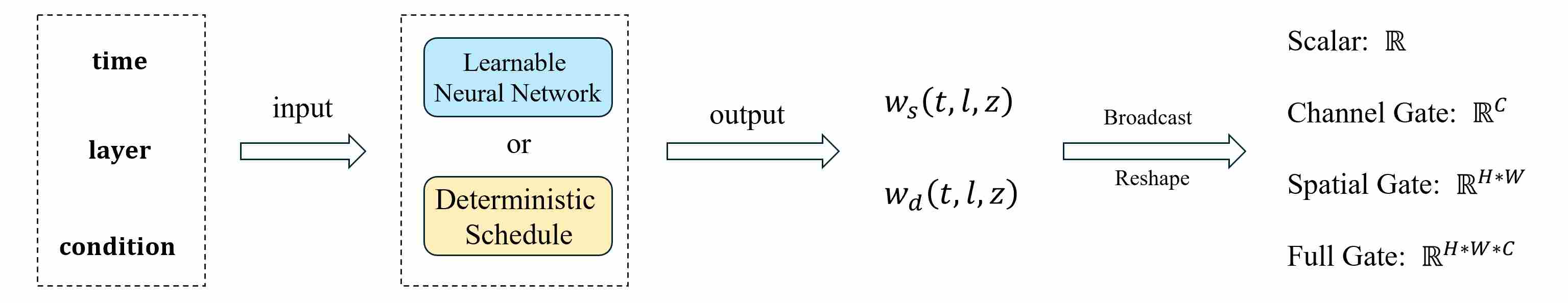
A practical design of $w_s$ / $w_d$ always consists of the following steps:
Step I. Choose the control inputs: what should the gate depend on?
Define a compact control vector $u$ from one (or more) of:
- Layer / hierarchy $\ell$ (resolution-level awareness): different scales require different skip strength.
- Timestep $t$ (SNR awareness): low SNR vs. high SNR regimes demand different routing.
- Condition $z$ (prompt/control awareness): different conditions should alter how much detail is passed.
In implementation, $u$ is often a concatenation of embeddings, e.g.
\[u = [\,e(t)\;;\; \mathrm{Emb}(\ell)\;;\; h(z)\,].\]Step II. Specify the mapping: learned gate vs. deterministic schedule. You then map $u$ to raw gate logits (or coefficients) using either:
- Learnable gates (small MLP / hypernetwork): expressive and condition-adaptive, but must be regularized / bounded.
- Deterministic schedules (hand-crafted, SNR-based, monotone): cheap, stable, interpretable, and often surprisingly effective.
Formally,
\[\tilde w_s = \psi(u),\qquad \tilde w_d=\psi'(u),\]where $\psi$ can be a neural network or a closed-form function.
Step III. Decide the output granularity: what tensor shape should the gate have?
The same mapping framework covers the common granularities:
- Scalar gate: $w\in\mathbb{R}$ → broadcast to $(1,1,1,1)$
- Channel gate: $w\in\mathbb{R}^{C_\ell}$ → reshape to $(1,C_\ell,1,1)$
- Spatial gate: $w\in\mathbb{R}^{H_\ell\times W_\ell}$ → reshape to $(1,1,H_\ell,W_\ell)$
- Full gate: $w\in\mathbb{R}^{C_\ell\times H_\ell\times W_\ell}$ → reshape to $(1,C_\ell,H_\ell,W_\ell)$
This is why many “different” skip weighting methods are actually the same recipe: they differ mainly in what goes into $u$ and what shape is emitted.
Step IV. Enforce stability: bounded parameterization + controlled gain.
Because long skips directly affect the Jacobian spectrum, the gate must prevent high-gain oscillations. In practice this means:
- Bound the gate: $w=\sigma(\tilde w)$ (or softplus/tanh variants) to avoid unbounded amplification.
- Variance-aware merge (optional but robust) for additive fusions: $$ y=\frac{w_d\,d + w_s\,s}{\sqrt{w_d^2+w_s^2+\epsilon}}, $$ which keeps feature scales controlled even when gates change across $t$ and $\ell$.
- Restrict risky granularities: spatial/full gates are powerful but can become sharp and unstable; they typically need smooth parameterizations and/or regularization.
Step V. Verify with diagnostics: “where does the learning signal go?”
A simple sanity check is to monitor feature/gradient balance across the two streams:
where $s’=w_s\odot\phi_s(s)$ and $d’=w_d\odot\phi_d(d)$. Extremely large ratios indicate skip dominance (shortcut learning / decoder starvation), motivating stronger suppression at low SNR or deep levels.
Takeaway. Designing $w_s$ and $w_d$ is not a collection of unrelated tricks; it is a unified pipeline: (choose inputs) $\to$ (choose mapping) $\to$ (choose granularity) $\to$ (broadcast + bounded modulation), whose goal is to keep skip routing hierarchy-aware, time-aware, condition-aware, and numerically controlled.
5.2 Mapping: From Control Signals to Weights (Learned vs. Deterministic)
In the unified formulation, the entire “weight / gate design” problem reduces to a mapping:
\[u(t,\ell,z)\ \xrightarrow{\ \psi\ }\ \tilde w\ \xrightarrow{\ \eta\ }\ w \ \xrightarrow{\text{broadcast}}\ w\odot (\cdot),\]where $u(t,\ell,z)$ is the control input (timestep / level / condition), $\psi$ produces a raw coefficient (or logits), $\eta$ enforces a stable parameterization (e.g., bounding or normalization), and the final $w$ is reshaped/broadcast to match the target feature tensor. This mapping view is already implicit in timestep-aware gating, where $w_s(t,\ell)$ can be implemented either as a learned MLP on $e(t)$ or as a simple deterministic schedule.
A learned gate typically uses a tiny network (MLP / hypernetwork) to map embeddings to coefficients:
\[\tilde w_s=\psi_s\big([e(t);\mathrm{Emb}(\ell);h(z)]\big),\qquad w_s=\eta(\tilde w_s).\]This is flexible and condition-adaptive, but it introduces a new failure mode: the gate itself can become high-gain and destabilize long-skip dynamics. Hence, the key engineering is not “which MLP,” but how to constrain $\eta(\cdot)$ and where to apply the gate (granularity/layers/timesteps).
Deterministic schedules instantiate the same mapping without learnable parameters: $w=\psi(t,\ell,z)$ is prescribed by closed-form rules or a small set of user-chosen scalars. They are attractive because they are fast, robust, interpretable, and often sufficient to fix the dominant stability issues (scale drift, timestep mismatch, skip dominance).
A. Variance / energy preserving schedules. For additive fusions, repeated merges can drift feature norms because
\[\mathrm{Var}(d+s)\approx \mathrm{Var}(d)+\mathrm{Var}(s)\]when the two streams are weakly correlated. A simple and effective remedy is to normalize the merge by its expected energy:
\[y=\frac{d+s}{\sqrt{2}} \quad\text{or more generally}\quad y=\frac{w_d\,d+w_s\,s}{\sqrt{w_d^2+w_s^2+\epsilon}}.\]This turns $(w_d,w_s)$ into “direction” parameters rather than “gain” parameters, preventing uncontrolled amplification even when weights change across $(t,\ell)$. This idea appears naturally in the variance-aware merge variant
\[y=\frac{d+\alpha_\ell s}{\sqrt{1+\alpha_\ell^2}},\]already used in the layer-wise scalar scaling discussion.
B. Layer-wise (hierarchy-aware) schedules. A large portion of stability issues can be addressed by prescribing a per-level coefficient $\kappa_\ell$ (or $\alpha_\ell$):
\[w_s(t,\ell,z)=\kappa_\ell,\qquad w_d(t,\ell,z)=1,\]or a normalized version via the energy-preserving merge above. The consensus for weighting skip connections ($w_s$) relative to network depth is the “Deep-Small, Shallow-Large” principle:
Deep Layers (Bottleneck & Low-Res): Small Weights (\(w_s \downarrow\)). The deep layers of the decoder are responsible for generating global structure and abstract semantics “from scratch” (based on the prompt/bottleneck).
If the skip connection weight is too large here, the decoder becomes “lazy,” relying on the encoder’s features instead of generating its own. Since encoder features at high noise levels are often unstructured or noisy, strong skip connections in deep layers cause semantic interference, leading to structural collapse or artifacts. Suppressing these weights forces the model to respect the bottleneck conditioning.
Shallow Layers (Input/Output & High-Res): Large Weights (\(w_s \uparrow\)) The shallow layers are responsible for reconstructing fine textures, edges, and pixel-level details.
Due to repeated downsampling, the bottleneck loses spatial precision. The decoder cannot hallucinate sharp edges without reference. Therefore, strong skip connections are crucial in shallow layers to transport high-frequency spatial information directly from the encoder, ensuring the final output is sharp and detailed rather than blurry.
Common deterministic parameterizations include:
- Piecewise stage constants: choose $(\kappa_{\text{deep}},\kappa_{\text{mid}},\kappa_{\text{shallow}})$ and assign by resolution groups.
- Monotone depth decay: $\kappa_\ell=\kappa_0\cdot r^{\ell}$ (exponential) or $\kappa_\ell=\kappa_0/(1+\lambda \ell)$ (rational), with $\ell$ increasing toward deeper blocks.
- Temperature-controlled sigmoid: $\kappa_\ell=\sigma\big(a(\ell-b)\big)$, useful when you want a smooth “transition depth.”
This family is conceptually aligned with “explicitly scale down long skip edges” (e.g., $\kappa_\ell$ or $\kappa_\ell(t)$) emphasized by the ScaleLong-style viewpoint.
C. Timestep / SNR-aware schedules. Because diffusion spans low-SNR (very noisy) to high-SNR (nearly clean) regimes, a constant skip strength cannot be optimal across time.
Design principle. A monotone schedule is often sufficient: suppress skip in low SNR (avoid noise leakage), and enable skip in high SNR (recover detail)
A deterministic schedule therefore uses a monotone function of noise level, e.g., $\mathrm{SNR}(t)$ (or $\log\mathrm{SNR}$, or $\sigma(t)$):
\[w_s(t,\ell)=\kappa_\ell\cdot g(\mathrm{SNR}(t)),\]where $g(\cdot)$ is chosen to suppress skip in low SNR (avoid noise leakage) and enable skip in high SNR (recover detail). Two practical deterministic forms:
- Sigmoid in log-SNR: with $(\beta,\tau)$ controlling sharpness and the “turn-on” point. $$ g(\mathrm{SNR})=\sigma\!\big(\beta(\log\mathrm{SNR}-\tau)\big), $$
- Clipped linear ramp: which is simple and highly interpretable $$ g(\mathrm{SNR})=\mathrm{clip}\Big(\frac{\log\mathrm{SNR}-\tau_0}{\tau_1-\tau_0},\,0,\,1\Big), $$
D. Condition-controlled but deterministic schedules. While fully condition-adaptive gating is usually learned, many practical systems expose a deterministic condition knob that scales skip injection, e.g., a user-chosen strength $\gamma(z)$ (ControlNet-like “control strength”, style strength, etc.):
\[w_s(t,\ell,z)=\gamma(z)\cdot \kappa_\ell\cdot g(\mathrm{SNR}(t)).\]This keeps the mapping deterministic while still allowing conditions to influence routing through an explicit, interpretable scalar. We tall about condition-aware control in section 8.
Takeaway. Mapping design is not about choosing a fancy gate network; it is about prescribing a stable function class for $w(t,\ell,z)$: hierarchy-aware ($\kappa_\ell$), time/SNR-aware ($g$), optionally condition-controlled ($\gamma$), and ideally variance-controlled via normalization.
5.3 Output Granularity: From Scalar to Full Gate
Let the aligned skip feature be
\[\tilde s=\phi_s(s)\in\mathbb{R}^{B\times C_\ell\times H_\ell\times W_\ell}\]and decoder feature
\[\tilde d=\phi_d(d)\in\mathbb{R}^{B\times C_\ell\times H_\ell\times W_\ell}\]at level \(\ell\). Then a gate is simply a tensor $g$ that is broadcastable to \((B,C_\ell,H_\ell,W_\ell)\), and applied as
\[y=\mathrm{Fuse}\big(\tilde d,\; g\odot \tilde s\big).\]So the “granularity choice” answers one question: what axes are allowed to vary?
| Gate type | Output space | Broadcasted shape at level (\ell) | What it can do best |
|---|---|---|---|
| Scalar gate | \(\mathbb{R}\) | \((B,1,1,1)\) | globally suppress/enable skip strength |
| Channel gate | \(\mathbb{R}^{C_\ell}\) | \((B,C_\ell,1,1)\) | select feature subspaces (edges/textures/semantics) |
| Spatial gate | \(\mathbb{R}^{H_\ell\times W_\ell}\) | \((B,1,H_\ell,W_\ell)\) | local routing / boundary-focused injection |
| Full gate | \(\mathbb{R}^{C_\ell\times H_\ell\times W_\ell}\) | \((B,C_\ell,H_\ell,W_\ell)\) | per-location and per-channel modulation |
Different granularities exert varying impacts on the stability of model training.
- Scalar Gates. A scalar gate is the most stable and cheapest option: it uniformly rescales the entire skip stream. This includes layer-wise coefficients \(\alpha_\ell\) and time-dependent scalars \(w_s(t,\ell)\) . Scalar gates are especially attractive when the primary goal is stability (preventing skip dominance, bounding feature norms, reducing gradient oscillation). When the fusion is additive, variance-aware rescaling (normalizing by \(\sqrt{1+\alpha_\ell^2}\)) keeps magnitudes bounded , and also mitigates the “variance drift” issue across repeated merges .
Channel Gates. Channel-wise gating is often a sweet spot: it is substantially more expressive than a scalar, while remaining much more stable than spatial/full masks :
\[y=\mathrm{Fuse}\big(\tilde d,\; g(t,\ell,z)\odot \tilde s\big),\qquad g\in\mathbb{R}^{C_\ell}.\]Why it works well in diffusion: channels tend to specialize (detail vs structure), so a channel gate can suppress “noisy detail channels” at low SNR without discarding all skip information . This directly targets timestep mismatch and reduces conflict between streams.
Spatial Gates. Spatial gating makes skip routing local :
\[y=\tilde d + m(t,\ell,z)\odot \tilde s,\qquad m\in\mathbb{R}^{H_\ell\times W_\ell}.\]It can dramatically improve controllability (e.g., emphasizing boundaries or regions), but it is also prone to instability: sharp/high-gain masks can amplify local gradients and create brittle optimization . In stability-oriented U-Nets, spatial gating is typically used with explicit smoothing/regularization or restricted to certain layers/timesteps .
- Full Gates. A full gate \(G\in\mathbb{R}^{C_\ell\times H_\ell\times W_\ell}\) allows every channel at every spatial location to be modulated differently. This is the most expressive setting, but it can easily become a high-gain long-skip amplifier, worsening the oscillatory / sensitive behavior induced by large long-skip coefficients . In diffusion U-Nets, full gates are usually justified only when you truly need dense, spatially varying modulation and you have strong stabilization measures (parameterization constraints, normalization, or architectural safeguards).
6. Stabilization via Transforms
Transforms $\phi$ address the representation mismatch: they align distributions, subspaces, and frequency content before fusion.
Linear projection: the default safe choice is \(1\times 1\) alignment with MLP projection:
\[\phi_s(s)=W_s * s,\qquad \phi_d(d)=W_d * d \quad (1\times1).\]Why it stabilizes. reduces channel-space incompatibility (learned rotation); can suppress harmful subspaces of the skip stream; makes fusion less sensitive to raw encoder anisotropy
Normalization: A robust template is to normalize both streams before fusion:
\[\phi_s(s)=\mathrm{Norm}(s),\qquad \phi_d(d)=\mathrm{Norm}(d),\]then apply weighting/fusion. This reduces amplitude mismatch and makes $w$ act more predictably.
Frequency-selective transforms: Frequency-selective transforms implement \(\phi_s\) by filtering or re-scaling specific spectral bands of the skip feature \(s\).
Let \(\mathcal{F}\) / \(\mathcal{F}^{-1}\) be the 2D Fourier transform / inverse transform (applied per channel). A frequency-selective skip transform can be written as
\[\phi_s(s)=\mathcal{F}^{-1}\!\big(\beta_{\ell,t}(\omega)\odot \mathcal{F}(s)\big),\]where \(\beta_{\ell,t}(\omega)\in\mathbb{R}\) is a (typically low-/high-band) spectral mask. Equivalently, with a two-band split,
\[s_{\text{low}}=\mathcal{F}^{-1}(M_{\text{low}}\odot \mathcal{F}(s)),\quad s_{\text{high}}=\mathcal{F}^{-1}(M_{\text{high}}\odot \mathcal{F}(s)),\]and \(\phi_s\) becomes band-wise scaling:
\[\phi_s(s)=\lambda_{\text{low}}(\ell,t)\,s_{\text{low}}+\lambda_{\text{high}}(\ell,t)\,s_{\text{high}}.\]This directly suppresses noise-prone bands (often high-frequency) at noisy steps, while preserving detail bands when SNR increases.
FreeU 10 applies a simple spectral edit to skip features (per level $\ell$, per channel), which is exactly an instance of \(\phi_s\):
\[\phi_s(s)=\mathrm{IFFT}\Big(\mathrm{FFT}(s)\odot \beta_{\ell}(\omega)\Big).\]Concretely, \(\beta_{\ell}(\omega)\) is a piecewise mask that downscales a selected frequency region by a factor \(s_\ell<1\) (and keeps the rest unchanged). Thus FreeU implements “frequency-selective attenuation” on the skip stream without changing the backbone parameters.
FreSca 11 formalizes the idea that scaling is more controllable when done per frequency band. With a low/high split, it rescales bands independently:
\[\widehat{x}=\mathcal{F}^{-1}\Big(\lambda_{\text{low}}\,M_{\text{low}}\odot \mathcal{F}(x)\;+\;\lambda_{\text{high}}\,M_{\text{high}}\odot \mathcal{F}(x)\Big).\]Although FreSca applies this to a diffusion signal $x$ (not necessarily a skip feature), the operator form matches \(\phi_s\) exactly: apply a band decomposition, then reweight low/high frequency components with separate coefficients.
Skip-Editor Transform: Instead of updating the whole U-Net or only LoRA on attention, another line emphasizes that skip pathways contain hierarchical information crucial for content and quality. It inserts lightweight tuners on skip edges:
\[\phi_s(s)=s+\mathrm{SC\text{-}Tuner}_\ell(s)\quad \text{(few parameters, localized training)}.\]Typical \(\mathrm{SC\text{-}Tuner}\) is a tiny neural network, it consists of a down module composed of CNNs and an up module composed of CNNs.
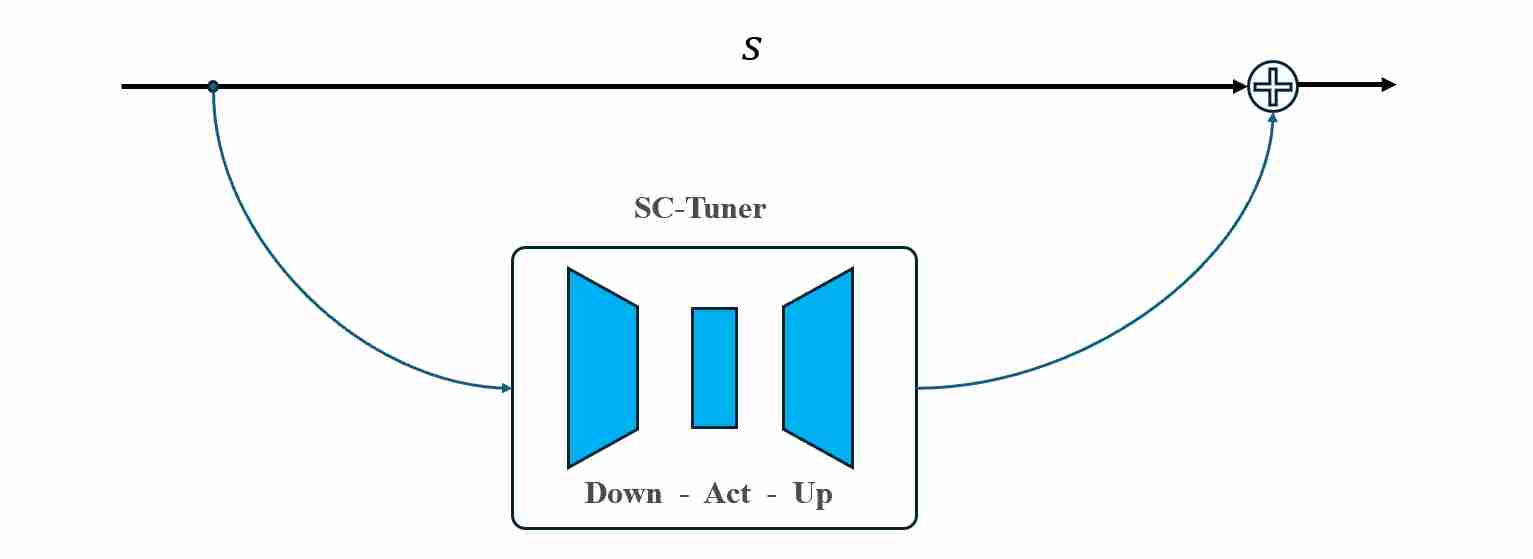 Figure 7: sc_tuner network
From the operator view, SCEdit primarily expands $\phi_s$ (and optionally couples it with condition $z$), creating a controllable and efficient adaptation interface.
Skip-Inject Transform: SkipInject-style methods 12, 13 show that certain encoder skip representations in Stable Diffusion carry strong spatial structure, enabling training-free editing/style transfer by injecting or swapping skip features:
Formally, at each resolution level (or selected encoder blocks) $\ell$, let $s_\ell(t)$ denote the skip feature produced by the current generation process, and \(s^{\text{ref}}_\ell(t)\) denote the skip feature extracted by running the same U-Net on a reference image (content/style/reference) at the same diffusion time $t$. SkipInject-style transforms define a reference-conditioned skip transform
\[\phi_s\big(s_\ell(t)\big)=\phi_s\big(s_\ell(t);\;s^{\text{ref}}_\ell(t)\big),\]where \(\phi_s\) is typically a simple, non-parametric operator such as replacement (swap):
\[\phi_s\big(s_\ell(t);\;s^{\text{ref}}_\ell(t)\big)=s^{\text{ref}}_\ell(t),\]or Linear injection (mixing):
\[\phi_s\big(s_\ell(t);\;s^{\text{ref}}_\ell(t)\big)=(1-\lambda_{\ell,t})\,s_\ell(t)+\lambda_{\ell,t}\,s^{\text{ref}}_\ell(t),\]or Residual injection:
\[\phi_s\big(s_\ell(t);\;s^{\text{ref}}_\ell(t)\big)=s_\ell(t)+\lambda_{\ell,t}\big(s^{\text{ref}}_\ell(t)-s_\ell(t)\big),\]
7. Stabilization via Fusion Operator
Fusion determines how gradients and variances couple across streams. In this chapter we assume the first two factors (weight and transform) have already been applied,
\[\tilde d \;\triangleq\; w_d(t,\ell,z)\odot \phi_d(d), \qquad \tilde s \;\triangleq\; w_s(t,\ell,z)\odot \phi_s(s),\]and we focus purely on the fusion operator:
\[y \;=\; \mathrm{Fuse}(\tilde d,\tilde s).\]In practice, most U-Net-like models fall into a small number of fusion families (additive, concatenative, attention-based, structured mixing).
Additive fusion: the naive fuse operation is addition
\[y = \tilde d + \tilde s\]
Concat fusion: defer coupling to a learnable mixer
\[y=\mathrm{Proj}([\tilde d;\tilde s]) \quad (\text{Proj: }1\times1\text{ conv or ResBlock}).\]
Attention fusion: A major source of instability in skip pathways is the semantic gap: encoder skip features can be “too local / too detailed”, while decoder features become increasingly semantic. Attention-based fusion makes the merge selective rather than unconditional.
\[\mathrm{Fuse}(\tilde d,\tilde s) = \tilde d \;+\; \mathrm{Attn}\Big(Q=\psi_Q(\tilde d),\;K=\psi_K(\tilde s),\;V=\psi_V(\tilde s)\Big).\]
Structured mixing fusion: Some works introduce fusion operators specifically to make the activation statistics of the two streams (skip feature and decoder feature) more compatible.
For example, in BI-DiffSR 14 (a binarized diffusion SR model), CS-Fusion shuffles channels across the two inputs before mixing, aiming to balance activation ranges and reduce distribution shift across timesteps. Abstractly, it can be written as:
\[[\hat d;\hat s] = \mathrm{Shuffle}([\tilde d;\tilde s]),\qquad y = h([\hat d;\hat s]),\]where \(\mathrm{Shuffle}\) is a fixed permutation and \(h\) is a lightweight mixing block.
8. Condition-Aware Routing Interfaces
Modern diffusion systems are condition-rich. A stability-centric statement is: Conditions should not only influence the output; they should influence the routing of information through skip pathways.
- If condition $z$ is strong and spatial (edges, depth, segmentation), the model should rely more on high-resolution detail pathways to maintain alignment.
- If condition $z$ is semantic (text style, high-level attributes), the model should avoid letting skip details override global semantics.
Without $z$-aware routing, the model must force all control into a single bottleneck/cross-attention interface, which often leads to: brittle composition of multiple conditions, unstable gradients when conditions compete, and unpredictable “over-control” or “under-control”
In operator form, this means $z$ should parameterize $w$, $\phi$, and sometimes Fuse:
\[w_s=w_s(t,\ell,z),\quad \phi_s=\phi_s(\cdot;z),\quad \mathrm{Fuse}=\mathrm{Fuse}(\cdot,\cdot;z).\]Stability principles for routing interfaces.
A routing interface is “stable” when it preserves the pretrained backbone behavior at initialization and limits gradient interference across pathways. Common patterns:- Identity-preserving initialization: start from “no-op” routing so the base U-Net behavior is unchanged (reduces early oscillations).
- Residual injection rather than replacement: inject $\Delta_\ell(z)$ additively, and optionally gate it by $(t,\ell)$.
- Backbone freezing / localized training: constrain learnable parameters to a small interface module to reduce distribution shift.
- Multi-scale alignment: map spatial conditions to matching resolutions (avoid forcing spatial control through low-resolution bottlenecks).
- Schedule-aware gating: allow routing strength to depend on $t$ (early steps may need global structure; late steps refine details).
ControlNet: stable conditional injection via zero-initialized connectors. 15
\[\bar s_\ell \;=\; s_\ell \;+\; \Delta_\ell(t,z), \qquad \Delta_\ell(t,z) \;=\; \mathrm{ZeroConv}_\ell\big(f^{\text{ctrl}}_\ell(x_t,t,z)\big),\]
ControlNet provides a branch-based interface for injecting a new condition (typically spatial control) without destabilizing a pretrained text-to-image U-Net. In the operator language, ControlNet can be viewed as expanding the skip stream through a zero-initialized residual:where \(f^{\text{ctrl}}_\ell\) denotes the ControlNet branch feature at level $\ell$, and $\mathrm{ZeroConv}_\ell$ is initialized to output zeros. This yields a strong stability guarantee at the start of training:
\[\mathrm{ZeroConv}_\ell(\cdot)\approx 0 \;\;\Rightarrow\;\; \bar s_\ell \approx s_\ell,\]so the base model’s behavior is preserved initially, and optimization learns a residual route rather than rewriting the skip pathway.
In terms of the unified decomposition, ControlNet primarily affects:
\[\phi_s(s;\,z)\approx s + \Delta(t,\ell,z),\]and in practice it is often paired with an explicit routing scale (a special case of $w_s(t,\ell,z)$) to avoid “control dominance”.
T2I-Adapter: lightweight condition alignment as $\phi(\cdot;z)$. 16
\[\bar s_\ell \;=\; s_\ell \;+\; \alpha_\ell(t)\odot e_\ell(z),\]
T2I-Adapter compresses the same idea into a lightweight multi-scale encoder that produces aligned condition features $e_\ell(z)$ and injects them into the U-Net at matching resolutions. A typical operator view is:where $\alpha_\ell(t)$ is a deterministic or learnable schedule (section 5). Compared to ControlNet, the adapter interface has smaller capacity, which often improves stability when data for the new condition is limited: it reduces the risk of the model learning a brittle bypass that overfits the control signal.
In unified-form terms, T2I-Adapter is best interpreted as a condition-dependent transform on the skip stream:
\[\phi_s(s;\,z)\;=\; s + \mathrm{Adapter}_\ell(z),\]with optional time/layer gating absorbed into $w_s(t,\ell,z)$.
SCEdit-style controllable skip tuners: editing via localized skip routing. 17
SCEdit makes the skip pathway itself a controllable interface by inserting small tuners on selected skip edges (or skip fusion sites). Its stability advantage is locality: the backbone can remain frozen while the tuner learns an edit-specific transformation.A generic operator form is:
\[\phi_s(s_\ell;\,z) \;=\; s_\ell \;+\; g_{\ell}(t,z)\odot T_\ell(s_\ell;\,z),\]where $T_\ell$ is a lightweight learnable module (few parameters) and $g_{\ell}(t,z)$ is a routing gate that decides where/when edits should take effect. This makes “editing strength” an explicit part of $w_s(t,\ell,z)$ and avoids uncontrolled global drift.
In a stability-centric reading, SCEdit is not “just controllability”: it is a concrete way to implement condition-aware routing that is (i) identity-friendly at initialization, and (ii) restricted to selected layers/timesteps to reduce interference with the base semantic computation.
Skip-Tuning: prompt-dependent routing by tuning a small set of skip controls. 18
\[w_s(t,\ell,z) \;=\; w_s^{\text{base}}(t,\ell)\cdot (1+\delta_{\ell}(z)),\]
Skip-Tuning highlights that surprisingly strong improvements can come from tuning only a small set of routing variables on skip pathways. In the unified notation, this can be expressed as optimizing (or learning) low-dimensional controls:where $\delta_{\ell}(z)$ is a small set of parameters (per-layer scalars or channel-wise scales). The key stability takeaway is that routing capacity can be separated from backbone capacity: adjusting skip routing can yield large effects while leaving the main computation intact.
Training-free routing: SkipInject / style injection as $z$-conditioned transforms. 12 13
\[\phi_s\big(s_\ell(t);\;z\big)=\phi_s\big(s_\ell(t);\;s^{\text{ref}}_\ell(t)\big),\]
Training-free methods show an extreme form of condition-aware routing: let $z$ be a reference image (style/content), extract reference skip features $s^{\text{ref}}_\ell(t)$, and definewith mixing strengths $\lambda_{\ell,t}$ acting as explicit routing schedules. From a stability viewpoint, these methods bypass optimization entirely and instead exploit the fact that skip pathways already encode rich, spatially aligned structure that can be “re-routed” at inference time.
In summary, section 5 to section 7 gave us the “local operator toolkit” for stabilizing skip fusion. This chapter adds the systems-level lesson: conditions should shape the routing policy of skip pathways. ControlNet, T2I-Adapter, and SCEdit illustrate three stable interface patterns—branch injection, lightweight aligned adapters, and localized skip tuners—that implement $z$-aware $w/\phi/\mathrm{Fuse}$ while preserving identity at initialization and limiting gradient interference. This perspective makes “controllability modules” directly relevant to architectural stability: they are not only about adding more conditions, but about adding them without destabilizing the skip operator.
9. Other U-Net Stability Designs
This chapter collects U-Net stability practices that do not fit cleanly into the skip operator decomposition, yet materially affect skip-pathway behavior and overall training stability.
Identity-friendly initialization for deep residual U-Nets.
A diffusion U-Net is extremely deep. A common stability pattern is to initialize residual branches so that each block starts close to an identity mapping (e.g., by zero-initializing the last conv in a residual branch). This reduces early training oscillations and helps gradients propagate, which indirectly prevents skip edges from becoming the only reliable pathway.
Restricting attention placement to avoid instability and cost spikes.
Self-attention blocks (and cross-attention in text-to-image) can destabilize training if placed at very high resolutions due to large token counts and large gradient variance. Many architectures restrict attention to mid/low resolutions, leaving high-resolution refinement to convolutional pathways (which includes skip pathways). This reduces the chance that high-resolution skips must compensate for unstable attention dynamics.
Up/downsampling choices and aliasing control.
The choice of up/downsampling (strided conv vs pooling vs resampling filters) affects the spectral content of features. If downsampling introduces aliasing, skip features can carry “incoherent high-frequency artifacts” that the decoder cannot reconcile stably. Anti-aliased resampling or carefully designed strided convs can improve stability, especially when combined with frequency-aware (\phi_s).
Regularizing bypass paths: skip dropout / stochastic routing (conceptual tool).
If skips become overly dominant, a conceptual countermeasure is to introduce stochasticity or dropout-like regularization on skip paths during training (carefully, to avoid quality collapse). This forces the backbone to remain competent and reduces the risk of a brittle bypass solution.
Part III — Stabilization in DiT Architectures
In diffusion / flow-matching DiTs, there are no long skip highways like U-Nets; instead, the backbone is a deep stack of homogeneous Transformer blocks, so the stability pressure is concentrated on per-block numerical stability under deep stacking. Consistent with the “unified operator” style used to open Part II, we describe each DiT block as a residual + multi-branch update operator:
\[h_{\ell+1} = h_\ell + \sum_{b\in\mathcal{B}_\ell} g_{\ell}^{(b)}(t,z)\odot F_{\ell}^{(b)}\Big( \mathrm{AdaLN}_{\ell}^{(b)}(h_\ell;\,t,z),\; c(z) \Big)\]The meanings of each symbol are summarized in the following table:
| Symbol | Meaning | Variation Dimensions |
|---|---|---|
| $h_\ell$ | Token features at Transformer block $\ell$ (e.g., patch/latent tokens) | Token + Channel |
| $\ell$ | Block (layer) index | Integer |
| $t$ | Diffusion timestep / continuous time | $[0,T]$ or $[0,1]$ |
| $z$ | External condition (class/text/style/control, etc.) | Modality / Type |
| $c(z)$ | Context sequence derived from $z$ (e.g., text tokens for cross-attn); optional / may be empty | Token-length + Channel |
| $\mathcal{B}_\ell$ | Set of update branches in block $\ell$ (e.g., SA / CA / MLP) | Architecture choice |
| $b$ | Branch index (e.g., $b!=!\text{sa},\text{ca},\text{mlp}$) | Discrete |
| $\mathrm{AdaLN}^{(b)}_\ell(\cdot;,t,z)$ | Conditioned normalization/modulation for branch $b$ (AdaLN / AdaLN-Zero variants) | Depends on $t,\ell,z$; design choice |
| $F^{(b)}_\ell(\cdot, c)$ | Branch operator (Self-Attn / Cross-Attn / MLP / etc.); uses $c(z)$ only when needed (e.g., cross-attn) | Operator type + parametrization |
| $g^{(b)}_\ell(t,z)$ | Gate / residual scaling for branch $b$ (controls update magnitude; often zero-init for stability) | Scalar / Channel / Head / Token; depends on $t,\ell,z$ |
| $\odot$ | Broadcastable elementwise modulation by the gate $g^{(b)}_\ell$ | Granularity-dependent |
10 Stabilization via Residual Scaling and Gates
In DiTs, every layer is a residual update, and there is no long-range skip highway like U-Net. As a result, stability is largely about controlling the magnitude of the per-block increment:
\[h_{\ell+1} \;=\; h_\ell \;+\; \Delta_\ell,\]with
\[\Delta_\ell \;=\;\sum_{b\in\{\text{attn},\text{mlp}\}} g_\ell^{(b)}(t,z)\odot F_\ell^{(b)}\!\Big(\mathrm{AdaLN}_\ell(h_\ell; t,z),\,c(z)\Big),\]where we treat residual scaling and gating as the primary “amplitude regulator” of \(\Delta_\ell\). This view is consistent with the DiT training philosophy that emphasizes identity-preserving residual behavior at initialization and controlled deviations thereafter 9.
10.1 Why residual amplitude must be regulated
A simple mental model is to assume the residual increments are roughly mean-zero and weakly correlated:
\[\mathbb{E}[\Delta_\ell]\approx 0, \qquad \mathbb{E}\|\Delta_\ell\|_2^2 \approx \sigma_\ell^2.\]Then the hidden-state energy grows with depth:
\[\mathbb{E}\|h_L\|_2^2 \;\approx\; \mathbb{E}\|h_0\|_2^2 \;+\;\sum_{\ell=0}^{L-1}\sigma_\ell^2.\]If \(\sigma_\ell\) does not shrink appropriately, deeper stacks drift into variance blow-up, which manifests as training instability, gradient spikes, or brittle conditioning.
So DiT-style stabilization often begins by answering a single question: How do we keep \(\|\Delta_\ell\|\) small early and controlled throughout training, while still allowing capacity later?
10.2 Deterministic residual scaling \(\beta_\ell\)
A clean way to make residual increments “scale-safe” is to insert an explicit depth scaling:
\[\Delta_\ell \;=\;\beta_\ell \sum_b \tilde g_\ell^{(b)}(t,z)\odot F_\ell^{(b)}(\cdot), \qquad \beta_\ell>0.\]Typical choices:
Constant scaling: \(\beta_\ell=\beta\).
A common heuristic is to set \(\beta\approx 1/\sqrt{2}\) when each block contains two additive sub-branches (attn + mlp), so their combined contribution stays bounded.Depth-dependent scaling: \(\beta_\ell \propto 1/\sqrt{L}\) (or slowly varying with \(\ell\)).
This matches the intuition that summing \(L\) increments of comparable scale should not cause \(\|h_L\|\) to grow as \(\sqrt{L}\) unchecked; related “depth-safe” residual parameterizations have been studied in very-deep Transformer scaling work 19.Small learnable scaling (LayerScale-style): initialize a per-channel scale to a tiny value (e.g., \(10^{-6}\) to \(10^{-4}\)), then learn it 20.
This starts the network extremely close to identity and gradually “opens up” capacity as training stabilizes.
These are architecture-level stabilizers: they do not depend on \(t\) or \(z\), and they primarily control depth accumulation risk.
10.3 Identity-preserving initialization: Zero-init and “start-as-identity” gates
The second pillar is to ensure that, at initialization,
\[h_{\ell+1}\approx h_\ell \quad\Longleftrightarrow\quad \Delta_\ell \approx 0.\]This can be implemented in several equivalent ways:
- Zero-init the last linear in each residual branch (so the branch output is initially near 0).
- Zero-init the gate (scalar or vector) that multiplies the branch output (ReZero-style gating) 21.
- AdaLN-Zero: generate gates (and often parts of modulation) from a zero-initialized projection, ensuring each block initially behaves as identity, then learns controlled deviations (DiT) 9.
In our unified view, all these are simply ways to make
\[g_\ell^{(b)}(t,z)\approx 0 \quad\text{(at init)} \quad\Rightarrow\quad \Delta_\ell \approx 0.\]10.4 Learned gates as “dynamic amplitude controllers”
Once deterministic scaling and identity initialization keep early training stable, learned gates become the main handle for adaptive stability:
\[g_\ell^{(b)}(t,z) \;=\; \underbrace{\beta_\ell}_{\text{depth safety}} \cdot \underbrace{\alpha_\ell^{(b)}(t,z)}_{\text{learned routing}}, \qquad \alpha_\ell^{(b)}(t,z)\in\mathbb{R}\ \text{or}\ \mathbb{R}^{C}.\]A good gate design typically satisfies:
- boundedness (avoid unbounded amplification), e.g. \(\alpha=\sigma(\cdot)\) or \(\alpha=\tanh(\cdot)\);
- granularity (scalar / per-branch / per-head / per-channel) matched to the instability mode;
- schedule-awareness (dependence on \(t\) or SNR), so the model does not inject overly aggressive updates when the input is mostly noise.
This naturally leads to the next chapters: gates and scaling are not isolated tricks; they interact strongly with modulation (AdaLN) and operator choice (attention/MLP).
11. Stabilization via Modulation Systems
In DiTs, modulation is not merely “conditioning injection”—it is the global controller that shapes the statistics of the signal entering each operator. In our notation, modulation is encapsulated by
\[u_\ell \;=\; \mathrm{AdaLN}_\ell(h_\ell; t,z), \qquad \Delta_\ell \;=\;\sum_b g_\ell^{(b)}(t,z)\odot F_\ell^{(b)}(u_\ell, c(z)).\]11.1 AdaLN as a closed-loop controller
A standard AdaLN form is:
\[\mathrm{AdaLN}(h; t,z) \;=\; (1+\gamma(t,z))\odot \mathrm{LN}(h) \;+\; \beta(t,z),\]where \(\gamma,\beta\) are produced by a small conditioning network (e.g., an MLP of time embedding and pooled text/class embedding) 9.
Stabilization intuition:
- LN normalizes feature scale token-wise, preventing operator inputs from drifting.
- \(\gamma,\beta\) then re-introduce controlled scale/shift aligned with \(t\) and \(z\).
- This turns conditioning into a regulated modulation rather than an unbounded additive perturbation.
11.2 AdaLN-Zero couples modulation with identity initialization
AdaLN-Zero augments the above by producing zero-initialized parameters (especially residual gates) so the block starts as identity:
\[\Delta_\ell \approx 0 \quad \text{initially},\]then, $\Delta_\ell$ increases only as learning discovers useful updates.
In practice, this acts like an “automatic warm-up” at the architectural level: the network begins in a stable regime without requiring extremely conservative optimization hyperparameters 9.
11.3 Norm placement: Pre-LN is a stability default
The most consequential architectural choice is often where normalization sits relative to residual addition:
- Pre-LN (typical in stable deep Transformers):
This preserves a clean gradient highway through the identity path 22.
- Post-LN:
which can entangle gradient scaling with the residual sum and may require warmup or careful tuning at large depth 22.
From the stability lens of diffusion backbones (deep stacks + multi-step training), Pre-LN + residual scaling + identity init is a particularly robust trio.
11.4 Beyond LN: RMS-style normalization as a pragmatic stabilizer
Large DiT variants sometimes replace or augment LN with RMS-style normalization (e.g., RMSNorm) in selected places, because it offers a simpler, often more stable scale control in practice:
\[\mathrm{RMSNorm}(x)= \frac{x}{\sqrt{\frac{1}{d}\sum_i x_i^2}+\epsilon}\odot w.\]This is particularly relevant when the main instability is logit saturation in attention (next chapter) 23.
12 Stabilization via Operator Design
Even with perfect scaling and modulation, the residual operator itself can introduce numerical pathologies. In our unified view, this is the stability contribution of the branch operators
\[F_\ell^{(\text{attn})}(\cdot),\qquad F_\ell^{(\text{mlp})}(\cdot).\]12.1 Attention: softmax saturation and logit explosion
Self-attention (and cross-attention) has the canonical form:
\[\mathrm{Attn}(Q,K,V)=\mathrm{softmax}\!\Big(\frac{QK^\top}{\sqrt{d_h}}\Big)V\]with \(Q,K,V\) learned projections 8.
Main stability risks:
- If \(\|Q\|\) or \(\|K\|\) grows, logits \(QK^\top/\sqrt{d_h}\) can become large, making softmax nearly one-hot → gradient starvation and brittle routing.
- Mixed-precision training amplifies sensitivity to extreme logits.
Common stabilizers:
- explicit scaling (the \(1/\sqrt{d_h}\) factor is essential);
- Q/K normalization (e.g., RMS-normalize \(Q,K\) per head before dot-product);
- cosine attention (normalize dot-product into a cosine similarity);
- logit clipping (cap attention logits before softmax).
From our unified lens, these are not “extra tricks”—they are ways of making \(F_\ell^{(\text{attn})}\) better behaved so the residual update \(\Delta_\ell\) remains well-conditioned.
12.2 MLP: activation dynamics and gated FFNs
The MLP branch usually takes:
\[F_\ell^{(\text{mlp})}(u)=W_2\,\phi(W_1 u),\]where \(\phi\) is an activation (GELU, SiLU, etc.). Instability can emerge from activation tails and feature-scale drift.
A widely adopted stabilizing alternative is gated FFNs (e.g., GLU/SwiGLU variants):
\[\mathrm{FFN}(u)=W_o\big(\phi(W_a u)\odot (W_b u)\big),\]which often yields better optimization and smoother dynamics 24.
In diffusion transformers, gated FFNs are particularly compatible with the “residual amplitude control” story: gating makes the effective residual update more selective and less likely to explode on hard/noisy timesteps.
12.3 Operator + residual coupling: where most failures actually occur
A practical observation is that many instabilities arise not from the operator alone, but from the composition
\[g_\ell^{(b)}(t,z)\odot F_\ell^{(b)}\Big(\mathrm{AdaLN}_\ell(\cdot),\,c(z)\Big).\]Hence, operator design should be evaluated together with:
- whether gates can suppress problematic updates,
- whether modulation keeps operator inputs normalized,
- whether residual scaling prevents accumulation across depth.
This motivates thinking in the unified equation rather than treating attention/MLP “in isolation.”
13. Stabilization via Conditional Routing: AdaLN vs Cross-Attn vs Joint-Attn
A key difference between U-Nets and DiTs is that conditioning is not a side branch; it directly shapes the residual operator through routing. In practice, modern DiT-style systems use three main conditioning interfaces.
13.1 Modulation-only routing (AdaLN as global control)
Mechanism: inject \(t,z\) through \(\gamma,\beta\) (and sometimes gates) in AdaLN:
\[u_\ell=\mathrm{AdaLN}_\ell(h_\ell;t,z).\]Stability profile:
- very stable (bounded modulation around normalized features),
- cheap (no extra token mixing),
- but limited for fine-grained token-level semantics.
This is why DiT class-conditioning can rely heavily on AdaLN/AdaLN-Zero: the condition is global and compact 9.
13.2 Cross-attention routing (token-level conditional mixing)
Mechanism: treat condition tokens as \(K,V\), and image tokens as \(Q\):
\[F_\ell^{(\text{cond-attn})}(u_\ell,z) =\mathrm{Attn}\big(Q=W_q u_\ell,\; K=W_k z,\; V=W_v z\big).\]Stability profile:
- very expressive (token-level alignment),
- but introduces an additional attention softmax and longer conditioning paths,
- often requires stronger normalization and/or gating to avoid early training collapse.
Many text-to-image DiT variants explicitly add cross-attention modules into DiT-like blocks for conditioning (e.g., PixArt-α) 25.
Important clarification: AdaLN and cross-attention are not mutually exclusive. A common stable division of labor is:
- AdaLN handles timestep + global style bias (cheap, stable),
- cross-attn handles token-level semantics (expressive, but stabilized by gates/norms).
13.3 Joint-attention / Multimodal DiT (MMDiT-style symmetric mixing)
Mechanism: concatenate image tokens and text tokens into a joint sequence, and apply a joint attention that allows bidirectional information flow:
\[[h;z] \;\mapsto\; \mathrm{Attn}([h;z]).\]A particularly influential design is to keep separate weights for each modality stream while sharing the attention interaction, enabling both “own-space processing” and cross-modal exchange 26.
Stability profile:
- improves text understanding and compositional binding by allowing image ↔ text token interaction at every layer,
- but increases the importance of attention stabilization (QK normalization, careful scaling, and gating),
- and makes schedule design over \(t\) and \(\ell\) even more critical (next chapter).
From the unified view, joint-attn mainly changes where \(z\) enters: instead of only modulating (AdaLN) or only serving as \(K,V\) (cross-attn), it becomes a first-class token stream inside the attention operator.
Part IV — Conclusion
Diffusion models succeed or fail not only because of losses, schedules, or optimizers, but because of their architectural choices. Across this article, we framed stability through two complementary levers: a control system that calibrates activations and embeds conditions (e.g., AdaGN/AdaLN), and signal pathways that govern how information flows (residual and skip routes). In U-Nets, stability is primarily about regulating skip fusion so shallow, high-variance details do not drown out deep semantics; in DiTs, which remove long skips, stability lives or dies by per-block design of normalization, residual scaling, and initialization. This separation of concerns explains why U-Nets emphasize skip regulation while DiTs emphasize normalization-centric residual design.
U-Net (encoder–decoder with long skips). Stable training relies on distributional alignment and amplitude regulation at fusion: normalize the skip, scale it, and re-normalize the sum to keep variance in check; then add gating (time/noise-aware, content-aware, or attention-based) so the network learns when and where detail should pass. Conditioning is most robust when implemented as modulation on normalization (AdaGN), which simultaneously stabilizes statistics and injects semantics across depth.
DiT (flat Transformer stacks). Without long skips, all gradient flow rides the residual branch, so architectural stability hinges on: (i) Pre-LN placement to preserve a direct gradient highway; (ii) residual scaling (e.g., (\beta!\approx!1/\sqrt{2})) to prevent variance blow-up across depth; (iii) identity-preserving initialization (Zero-Init / AdaLN-Zero) so each block starts near an identity in forward and backward passes; and (iv) gated FFN variants to tame activation dynamics.
A practical checklist for stability-oriented design.
- Choose normalization as a controller, not a patch. Use GN/AdaGN in U-Nets (small batches, per-sample stability), AdaLN in DiTs; prefer Pre-LN in Transformers to keep gradients well-conditioned across hundreds of layers.
- Regulate additive paths. For U-Net skips, apply (normalize → scale → renormalize); for residuals in any backbone, use explicit scaling (e.g., (\beta)) to avoid cumulative variance growth.
- Gate by signal quality. Make skip (or residual) contribution a function of timestep/SNR and content, so high-noise states don’t leak clutter and low-noise states pass crisp detail.
- Start from identity. Zero-init residual-path scalars (AdaLN-Zero) to ensure early-training stability, then learn controlled deviations from identity.
Broader lesson. Stability is an emergent property of architecture–conditioning–noise-schedule co-design. Treat normalization as the global controller, and treat skip/residual pathways as regulated channels whose variance and semantics must be balanced. In U-Nets this means fusing cautiously; in DiTs it means stacking safely.
Looking ahead. Promising directions include: (i) hybrid backbones that marry U-Net multi-scale inductive biases with Transformer token-level global reasoning; (ii) tighter architecture–preconditioning coupling for different noise parameterizations; and (iii) stability-aware lightweighting (gated residuals, linearized attention, and teacher-guided distillation) to push the Pareto frontier of fidelity vs. efficiency.
By elevating stability to a first-class architectural goal—and by applying the concrete rules distilled here—practitioners can scale diffusion systems more reliably, and researchers can explore deeper, broader, and more conditioned models without trading away robustness.
Part V — References
Ronneberger O, Fischer P, Brox T. U-net: Convolutional networks for biomedical image segmentation[C]//International Conference on Medical image computing and computer-assisted intervention. Cham: Springer international publishing, 2015: 234-241. ↩ ↩2
Ho J, Jain A, Abbeel P. Denoising diffusion probabilistic models[J]. Advances in neural information processing systems, 2020, 33: 6840-6851. ↩
Dhariwal P, Nichol A. Diffusion models beat gans on image synthesis[J]. Advances in neural information processing systems, 2021, 34: 8780-8794. ↩
Perez E, Strub F, De Vries H, et al. Film: Visual reasoning with a general conditioning layer[C]//Proceedings of the AAAI conference on artificial intelligence. 2018, 32(1). ↩
Brock A, Donahue J, Simonyan K. Large scale GAN training for high fidelity natural image synthesis[J]. arXiv preprint arXiv:1809.11096, 2018. ↩
Rombach R, Blattmann A, Lorenz D, et al. High-resolution image synthesis with latent diffusion models[C]//Proceedings of the IEEE/CVF conference on computer vision and pattern recognition. 2022: 10684-10695. ↩
Podell D, English Z, Lacey K, et al. Sdxl: Improving latent diffusion models for high-resolution image synthesis[J]. arXiv preprint arXiv:2307.01952, 2023. ↩
Vaswani A, Shazeer N, Parmar N, et al. Attention is all you need[J]. Advances in neural information processing systems, 2017, 30. ↩ ↩2
Peebles W, Xie S. Scalable diffusion models with transformers[C]//Proceedings of the IEEE/CVF international conference on computer vision. 2023: 4195-4205. ↩ ↩2 ↩3 ↩4 ↩5 ↩6
Si C, Huang Z, Jiang K, et al. FreeU: Free Lunch in Diffusion U-Net[C]//Proceedings of the IEEE/CVF Conference on Computer Vision and Pattern Recognition. 2024: 4733-4743. ↩
Huang C, Liang S, Tang Y, Bi J, Ma L, Tian Y, Xu C. FreSca: Scaling in Frequency Space Enhances Diffusion Models[J]. arXiv preprint arXiv:2504.02154, 2025. ↩
Schaerf L, Alfarano A, Silvestri F, et al. Training-Free Style and Content Transfer by Leveraging U-Net Skip Connections in Stable Diffusion[J]. arXiv preprint arXiv:2501.14524, 2025. ↩ ↩2
Chung J, Hyun S, Heo J P. Style injection in diffusion: A training-free approach for adapting large-scale diffusion models for style transfer[C]//Proceedings of the IEEE/CVF conference on computer vision and pattern recognition. 2024: 8795-8805. ↩ ↩2
Chen Z, Qin H, Guo Y, et al. Binarized diffusion model for image super-resolution[J]. Advances in Neural Information Processing Systems, 2024, 37: 30651-30669. ↩
Zhang L, Agrawala M. Adding Conditional Control to Text-to-Image Diffusion Models[C]//Proceedings of the IEEE/CVF International Conference on Computer Vision. 2023: 3813-3824. ↩
Mou C, Wang X, Xie L, et al. T2I-Adapter: Learning Adapters to Dig out More Controllable Ability for Text-to-Image Diffusion Models[J]. arXiv preprint arXiv:2302.08453, 2023. ↩
Jiang Z, Chen Y, Ye P, et al. SCEdit: Efficient and Controllable Image Diffusion Generation via Skip Connection Editing[C]//Proceedings of the IEEE/CVF Conference on Computer Vision and Pattern Recognition. 2024: 8995-9004. ↩
Ma J, Xue S, Hu T, et al. The Surprising Effectiveness of Skip-Tuning in Diffusion Sampling[C]//International Conference on Machine Learning. PMLR, 2024: 34053-34074. ↩
Wang H, Ma S, Dong L, et al. DeepNet: Scaling Transformers to 1,000 Layers[J]. arXiv preprint arXiv:2203.00555, 2022. ↩
Touvron H, Cord M, Sablayrolles A, et al. Going Deeper with Image Transformers[C]//Proceedings of the IEEE/CVF International Conference on Computer Vision. 2021: 32-42. ↩
Bachlechner T, Majumder B P, Mao H H, et al. ReZero is All You Need: Fast Convergence at Large Depth[C]//Proceedings of the Thirty-Seventh Conference on Uncertainty in Artificial Intelligence. PMLR, 2021: 1352-1361. ↩
Xiong R, Yang Y, He D, et al. On Layer Normalization in the Transformer Architecture[C]//International Conference on Machine Learning. PMLR, 2020. ↩ ↩2
Zhang B, Sennrich R. Root Mean Square Layer Normalization[J]. arXiv preprint arXiv:1910.07467, 2019. ↩
Shazeer N. Glu variants improve transformer[J]. arXiv preprint arXiv:2002.05202, 2020. ↩
Chen J, Yu J, Ge C, et al. PixArt-α: Fast Training of Diffusion Transformer for Photorealistic Text-to-Image Synthesis[J]. arXiv preprint arXiv:2310.00426, 2023. ↩
Esser P, Kulal S, Blattmann A, et al. Scaling Rectified Flow Transformers for High-Resolution Image Synthesis[J]. arXiv preprint arXiv:2403.03206, 2024. ↩