
Diffusion Architectures Part II: Efficiency-Oriented Designs
Published:
📚 Table of Contents
In the previous article, we examined architectural strategies for stability, contrasting how U-Nets and DiTs differ in their design philosophies and failure modes. In this article, we shift the focus to efficiency — how diffusion architectures can be restructured to accelerate computation and reduce memory usage, both during training and inference.
Efficiency here is not limited to faster math; it spans multiple layers of architectural design. At the representation level, latent diffusion and cascade models reduce the spatial or temporal burden of generation. At the backbone level, lightweight convolutional blocks, optimized feed-forward networks, and refined skip/normalization schemes streamline UNets and DiTs. At the attention level, sparse, kernelized, and FlashAttention variants tackle the quadratic bottleneck directly. Finally, at the system level, techniques such as activation checkpointing, ZeRO, quantization, and KV-cache optimization minimize memory footprint while sustaining throughput.
These efficiency-oriented designs fundamentally reshape the accessibility of diffusion models. By lowering both computational and memory costs, they make large-scale training feasible, real-time inference practical, and edge deployment attainable.
1. Introduction
Diffusion models have rapidly evolved from research prototypes to the foundation of modern generative systems in vision, language, and multi-modal applications. Their success, however, comes at a cost: diffusion models are notoriously resource-intensive. Training requires hundreds of GPU days, inference often takes dozens of steps to produce a single image, and deployment on memory-constrained or latency-sensitive platforms is still challenging. As a result, efficiency optimization has emerged as a central research and engineering problem.
1.1 Scope of This Article
This article focuses specifically on architectural efficiency in diffusion models. Here, our attention is restricted to the core design of the model architecture — how the network is built and executed during training and inference. We frame efficiency along two orthogonal axes:
- Computation Acceleration: Reducing FLOPs, bandwidth, or latency without sacrificing output quality.
- Memory Optimization: Minimizing GPU memory footprint, both in forward/backward passes during training and in caching/quantization during inference.
1.2 Dimensions of Optimization
We organize the efficiency landscape into four major parts:
- Representation-Level Efficiency: Reducing the problem size through latent spaces, cascades, and multi-resolution design.
- Backbone and Building Blocks: Lightweight convolutions, streamlined feed-forward networks, normalization refinements, and dynamic computation strategies in UNet/DiT backbones.
- Efficient Attention: From sparse/local to kernelized and FlashAttention, attention remains the primary bottleneck in both compute and memory.
- System-Level Memory Efficiency: Training-time methods such as checkpointing and ZeRO, and inference-time methods such as KV cache optimization and quantization.
Together, these dimensions cover the end-to-end lifecycle of efficiency in diffusion models: from training scalability to inference deployment, always through the lens of architectural design.
2. Representation-Level Efficiency Design
A unifying principle behind efficiency-oriented architectures is to avoid running the full diffusion process at full pixel resolution. Since the cost of convolutions and attention grows rapidly with spatial size, denoising directly in pixel space becomes prohibitive at high resolutions. Two dominant strategies address this challenge: (i) latent diffusion, which compresses images into a smaller latent space and performs the entire diffusion process there; and (ii) multi-stage cascades, which decompose generation into multiple diffusion stages of increasing resolution. Both approaches drastically reduce computation, but they differ in how the process is structured.
2.1 Latent Diffusion
A key leap in efficiency came with Latent Diffusion Models (LDMs) 1. Instead of applying the diffusion process directly on pixel space $\mathbf{x} \in \mathbb{R}^{H \times W \times 3}$, which is computationally expensive, an autoencoder first maps images into a compressed latent space:
\[\mathbf{z} = \mathcal{E}(\mathbf{x}), \quad \mathbf{x} \approx \mathcal{D}(\mathbf{z}),\]where $\mathcal{E}$ and $\mathcal{D}$ are encoder–decoder pairs trained with perceptual and adversarial losses. The diffusion process then operates on $\mathbf{z} \in \mathbb{R}^{h \times w \times c}$, with $h = H/f, \; w = W/f$, and $f$ is the downsampling factor. This reduces computation approximately by
\[\text{FLOPs}_{\text{latent}} \approx \frac{1}{f^2} \cdot \text{FLOPs}_{\text{pixel}},\]while maintaining perceptual quality through a powerful decoder. In practice, Stable Diffusion achieves up to 16–64× savings compared to pixel-space diffusion.
- Strength: The entire denoising process happens in a single latent space, greatly reducing FLOPs and memory, while preserving semantics.
- Weakness: Performance is tied to the quality of the autoencoder; poor reconstruction leads to artifacts.
2.2 Multi-Stage Cascades: Resolution-Based and SNR-Based Design
Training a single diffusion model to perform high-fidelity generation across all scales and noise levels is extremely challenging. The data distribution evolves drastically as the signal-to-noise ratio (SNR) decreases—early steps correspond to highly noisy inputs dominated by global semantics, while late steps focus on fine-grained textures. To handle this large dynamic range, modern diffusion architectures often adopt multi-stage cascades, which decompose the generation process into multiple specialized models. These cascades can be organized along two orthogonal axes: Resolution-Based Cascades and SNR-Based Cascades.
2.2.1 Resolution-Based Cascades
A Resolution-Based Cascade divides the generation task by spatial scale 2. They split generation into multiple independent diffusion stages, each operating at progressively higher resolutions: a base model first synthesizes a coarse, low-resolution image that captures the global layout and semantics. Then, one or more refiner models progressively upsample and enhance the result to higher resolutions, injecting local detail and texture fidelity at each stage.
Formally, Let \(\mathbf{x}_T\) denote the target high-resolution image and \(\mathbf{x}_{\ell}\) a lower-resolution intermediate representation. A cascade decomposes the marginal distribution into
\[p(\mathbf{x}_T)\, \approx\, p_{\theta}^{\text{base}}(\mathbf{x}_{\ell})\, \cdot\, p_{\phi}^{\text{ref}}(\mathbf{x}_T \mid \mathbf{x}_{\ell})\]where $p_{\theta}^{\text{base}}$ is modeled by a base diffusion model trained at low resolution, and $p_{\phi}^{\text{ref}}$ is one or more refiner diffusion models trained at higher resolutions conditioned on the base output. This decomposition follows the intuition that global semantic layout can be captured at coarse scales, while high-frequency detail is injected only where necessary.
1️⃣ Training objectives
Both the base and refiner are trained with standard denoising objectives, but differ in their conditioning.
Base stage. Operates at low resolution $(H_\ell, W_\ell)$. The training objective follows the conventional denoising score-matching loss:
\[\mathcal{L}_{\text{base}} = \mathbb{E}_{\mathbf{x}, t, \epsilon}\Big[\|\epsilon - \epsilon_{\theta}(\mathbf{x}_t, t)\|_2^2\Big]\]where \(\mathbf{x}_t\) is the noised low-resolution image and \(\epsilon_{\theta}\) predicts the corruption noise.
Refiner stage. Operates at higher resolution $(H, W)$. Its denoising network is conditioned on an upsampled version of the base output, \(\mathbf{c} = \phi(\text{Up}(\mathbf{x}_{\ell}))\), where $\phi(\cdot)$ is a learnable encoder, $\mathbf{x}_{\ell}$ is the output of based model. The conditional loss becomes:
\[\mathcal{L}_{\text{ref}} = \mathbb{E}_{\mathbf{x}, t, \epsilon}\Big[\|\epsilon - \epsilon_{\phi}(\mathbf{x}_t, t, \mathbf{c})\|_2^2\Big].\]Conditioning can be injected via concatenation of features or through cross-attention layers:
\[\text{CrossAttn}(\mathbf{Q}, \mathbf{K}, \mathbf{V}) \;=\; \text{softmax}\!\left(\tfrac{\mathbf{Q}\mathbf{K}^\top}{\sqrt{d}}\right)\mathbf{V},\]where queries $\mathbf{Q}$ derive from the high-resolution denoising stream and keys/values $\mathbf{K},\mathbf{V}$ from the encoded base output.
2️⃣ Inference procedure
At inference, all stages are executed in sequence
the base model first generates a low-resolution image \(\hat{\mathbf{x}}_{\ell}\) using many diffusion steps \(S_{\text{base}}\), which is computationally inexpensive due to the reduced spatial size.
This coarse sample is then upsampled and encoded as condition \(\hat{\mathbf{c}} = \phi(\text{Up}(\hat{\mathbf{x}}_{\ell}))\). The refiner then runs a conditional diffusion process with fewer steps \(S_{\text{ref}} \ll S_{\text{base}}\), focusing on the fine-detail portion of the noise schedule:
\[\hat{\mathbf{x}}_{t-1} = \mathcal{G}_{\phi}(\hat{\mathbf{x}}_{t}, t, \hat{\mathbf{c}}), \quad t=S_{\text{ref}},\dots,1.\]
2.2.2 SNR-Based Cascade
While resolution-based cascades divide the generation process spatially, an alternative strategy is to separate the diffusion process along the noise scale, or equivalently, the signal-to-noise ratio (SNR) 3. In this design, models are specialized for different SNR ranges rather than different image resolutions.
Specifically, a base model is trained to handle the high-noise (low-SNR) region of the diffusion process, where the input is close to pure Gaussian noise and the task primarily involves reconstructing the coarse global structure of the image. A second refiner model focuses on the low-noise (high-SNR) region, where the model’s objective shifts toward recovering subtle textures, colors, and fine-grained details.
During inference, the denoising trajectory is explicitly divided into two SNR regimes. The base model is used to sample from the noisy region down to an intermediate noise level, and the refiner then continues the sampling process until a clean image is obtained:
\[x_{t_k} \xrightarrow[\text{base model}]{\text{high noise}} x_{t_m} \xrightarrow[\text{refiner model}]{\text{low noise}} x_{0}.\]This approach effectively decouples the learning difficulty across the diffusion time domain. High-noise stages benefit from a model that focuses on structural reconstruction and semantic consistency, while low-noise stages leverage a separate model that is better conditioned for detailed restoration. Empirically, such division leads to more stable training and better overall visual fidelity, as each network only needs to learn a narrower, well-conditioned subset of the diffusion trajectory.
Notably, SNR-based cascades can be applied independently of resolution scaling, or combined with a resolution-based design. For example, SDXL and PixArt models employ a hybrid configuration, where the base model operates at a lower resolution and higher noise levels, while the refiner operates at a higher resolution and lower noise levels, unifying the benefits of both strategies.
2.2.3 Summary
Although these two strategies are conceptually independent, modern diffusion architectures often combine both cascades. For example, the SDXL and Stable Diffusion 3 pipelines employ a low-resolution, high-noise base model and a high-resolution, low-noise refiner, unifying the strengths of both spatial and noise-level specialization.
| Cascade Type | Division Axis | Focus Region | Primary Objective | Representative Models | Key Advantages |
|---|---|---|---|---|---|
| Resolution-Based | Spatial resolution | From low-res → high-res | Progressive upsampling and texture refinement | Imagen, SDXL, SD3 | Efficient training, better spatial detail |
| SNR-Based | Noise level (SNR/time) | From high-noise → low-noise | Stable denoising and detail recovery | SDXL, PixArt-δ, Flux.1 | Improved stability, better fine detail reconstruction |
In summary, Resolution-Based Cascades specialize across space, while SNR-Based Cascades specialize across time (noise level). Combining both axes yields a two-dimensional hierarchy that efficiently balances training stability, visual fidelity, and computational scalability, forming the foundation for modern high-quality diffusion systems.
2.3 Multi-Resolution Strateries
Multi-Stage Cascades distribute the generative process across multiple separate diffusion models, each trained and run at different resolutions (e.g., base 64×64 → refiner 256×256 → super-res 1024×1024). By contrast, Multi-Resolution strategies are applied inside a single model: the network itself processes features at multiple resolutions, progressively downsampling to capture global context and upsampling to recover details. In other words:
- Cascades = multi-resolution across models (pipeline of diffusion models).
- Multi-Resolution = multi-resolution within one model (hierarchical encoder/decoder or token pyramid).
Both reduce computation by avoiding full-resolution processing throughout the entire network, but multi-resolution design is intra-model and executed in a single forward pass.
2.3.1 Motivation for hierarchical design
There are two principal reasons why hierarchical processing is indispensable:
Time/Memory Complexity: for an image of size $H \times W$, the complexity of a Convolutional layer is
\[\text{FLOPs}_{\text{conv}} \;\sim\; H W \, k^2 \, C_{\text{in}} C_{\text{out}}\]where $k$ is kernel size, Downsampling by a factor of two reduces convolutional cost by 4x. while self-attention scales quadratically
\[\text{FLOPs}_{\text{attn}} \;\sim\; \mathcal{O}( (H W)^2\,d)\]Downsampling by a factor of two reduces convolutional cost by 16x. Thus, processing deep layers at coarser resolutions yields large savings in both time and memory.
Global Receptive Field: High-resolution convolutions have local receptive fields. Without downsampling, deep layers struggle to integrate global structures (object layout, long-range dependencies). Multi-resolution hierarchies solve this: downsampling reduces spatial size, so even small kernels or limited attention span can cover the entire image.
2.3.2 U-Net: inherently multi-resolution
The U-Net architecture embodies multi-resolution by design. Let the feature map at level (s) be
\[\mathbf{f}_s = \mathcal{E}_s(\mathbf{f}_{s-1}), \quad H_s = \tfrac{H}{2^s}, \; W_s = \tfrac{W}{2^s}.\]At the bottleneck $s=S$, the receptive field spans the entire input. During decoding, upsampled features $\text{Up}(\mathbf{y}s)$ are fused with encoder features $\mathbf{f}{s-1}$ via
\[\mathbf{y}_{s-1} = \phi\,\big(\text{Up}(\mathbf{y}_s) \oplus \mathbf{f}_{s-1}\big)\]where $\oplus$ denotes concatenation or addition. This design simultaneously achieves global awareness (via coarse levels) and local precision (via skip connections). For U-Net, multi-resolution is not optional—it is the fundamental mechanism enabling both efficiency and fidelity.
2.3.3 DiT: single-scale by default, multi-resolution as an extension
Diffusion Transformers (DiTs) typically follow a homogeneous, single-scale design, operating on a fixed token sequence of length
\[N = \frac{H}{p}\cdot \frac{W}{p}, \quad \mathbf{X}_0 \in \mathbb{R}^{N \times d}.\]where $p$ is the patch size. Attention layers in this setting have complexity \(\mathcal{O}(N^2 d)\), which becomes prohibitive for large (H,W). While global context is naturally available via full self-attention, efficiency suffers.
Some transformer variants also attempt to adopt the multi-resolution hierarchical architecture, such as swin transformer 4. There are several different ways to introduce multi-resolution
Hierarchical Patch Merging (pyramidal DiT). At stage $s$:
\[N_s = \frac{N_{s-1}}{4}, \quad d_s = 2\,d_{s-1}, \quad \mathbf{X}_s = \mathsf{M}_s\,(\mathbf{X}_{s-1})\]where $\mathsf{M}_s$ merges $2 \times 2$ neighboring tokens. This reduces token count, lowering attention cost by up to 16x per stage, while increasing channel dimension for expressiveness.
Token Pooling / Dynamic Selection. Select only (M \ll N) tokens based on saliency scores (s_i = g(\mathbf{x}_i)), then run attention/MLPs on the reduced set.
2.3.4 Summary
U-Net: Multi-resolution is essential, simultaneously lowering complexity and enabling global context capture.
DiT: Single-scale self-attention already provides global dependencies, but incurs quadratic cost; hierarchical designs are therefore optional but highly beneficial at high resolution.
Comparison with cascades: Multi-resolution strategies internalize hierarchy within a single model, whereas cascades externalize it across multiple models. Both can be combined for further gains.
3. Backbone-Level Architectures Design
Beyond operating at reduced resolutions, another path to efficiency is to redesign the fundamental building blocks of diffusion backbones. Convolution and attention are the two dominant computational modules: U-Net–based architectures rely heavily on convolutions, while Transformer-based DiTs are dominated by self-attention. Both can be optimized for efficiency without severely compromising quality.
3.1 UNet-Oriented Optimizations
In U-Net style backbones, most computation comes from repeated $3\times3$ convolutions. A standard convolution of kernel size $K$ with input channels $C_{\text{in}}$ and output channels $C_{\text{out}}$ has cost:
\[\text{FLOPs}_{\text{conv}} = H \cdot W \cdot K^2 \cdot C_{\text{in}} \cdot C_{\text{out}}.\]The number of parameters is:
\[\text{Param}_{\text{conv}} = K^2 \cdot C_{\text{in}} \cdot C_{\text{out}}\]To reduce cost, several lightweight alternatives are widely adopted.
3.1.1 Parameter and Computation Reduction
The goal is to reduce FLOPs and parameter count while maintaining accuracy.
A: Depthwise-Separable Convolution
Depthwise-separable convolution 5 6 decomposes a standard convolution into two lightweight components:
depthwise convolution: that applies a single spatial filter per input channel. specifically, each input channel is filtered independently with a spatial kernel of size $ K \times K \times 1 $. The output remains $ C_{\text{in}} $ channels. The computational cost (in FLOPs) and the number of parameters are:
\[\text{FLOPs}_{\text{dw}} = H' \cdot W' \cdot K^2 \cdot C_{\text{in}},\qquad \text{Param}_{\text{dw}} = K^2 \cdot C_{\text{in}}\]pointwise convolution: A 1×1 convolution is applied to project the $ C_{\text{in}} $-channel feature map into $ C_{\text{out}} $ channels. The computational cost (in FLOPs) and the number of parameters are:
\[\text{FLOPs}_{\text{pw}} = H' \cdot W' \cdot C_{\text{in}} \cdot C_{\text{out}},\qquad \text{Param}_{\text{pw}} = C_{\text{in}} \cdot C_{\text{out}}\]The total computational cost (in FLOPs) and the total number of parameters are:
\[\begin{align} & \text{FLOPs}_{\text{seq}} = \text{FLOPs}_{\text{dw}} + \text{FLOPs}_{\text{pw}} = H' \cdot W' \cdot \left( K^2 \cdot C_{\text{in}} + C_{\text{in}} \cdot C_{\text{out}} \right) \\[10pt] & \text{Param}_{\text{seq}} = \text{FLOPs}_{\text{dw}} + \text{FLOPs}_{\text{pw}} = K^2 \cdot C_{\text{in}} + C_{\text{in}} \cdot C_{\text{out}} \end{align}\]The relative computational reduction compared to standard convolution is:
\[\frac{\text{FLOPs}_{\text{seq}}}{\text{FLOPs}_{\text{conv}}} \approx \frac{1}{C_{\text{out}}} + \frac{1}{K^2}\]For typical values (e.g., $ K=3, C_{\text{out}} \geq 64 $), this yields more than 85% reduction in FLOPs.
B: Group Convolution
Divide the input channel and the output channel into $g$ groups, and convolution is only computed within each groups separately. The total computational cost (in FLOPs) and the total number of parameters are:
\[\begin{align} & \text{FLOPs}_{\text{group}} = H' \cdot W' \cdot \left( K^2 \cdot \frac{C_{\text{in}} \cdot C_{\text{out}}}{g} \right) \\[10pt] & \text{Param}_{\text{group}} = K^2 \cdot \frac{C_{\text{in}} \cdot C_{\text{out}}}{g} \end{align}\]C: Spatially Separable Convolution
Decomposes a $K \times K$ convolution into a sequence of a $K \times 1$ convolution followed by a $1 \times K$, particularly for factorizing larger kernels like $7 \times 7$ to reduce computational cost.
\[\begin{align} & \text{FLOPs}_{\text{group}} = H' \cdot W' \cdot \left( (2K) \cdot \frac{C_{\text{in}} \cdot C_{\text{out}}}{g} \right) \\[10pt] & \text{Param}_{\text{group}} = (2K) \cdot \frac{C_{\text{in}} \cdot C_{\text{out}}}{g} \end{align}\]3.1.2 Efficient Block Design
The goal is to design modular blocks that improve efficiency beyond basic convolutions.
A: ResNet Bottleneck
The bottleneck block was introduced in ResNet-50/101/152 7 to reduce the cost of stacking very deep networks. Instead of applying a full $3\times3$ convolution over $C$ channels (which costs $O(C^2k^2)$), the bottleneck design compresses the channel dimension first, performs spatial convolution in a reduced space, and then expands back. Bottleneck is act as a “wide -> narrow -> wide” channel structure, the workflow of bottleneck is shown as follows.

The total computational cost (in FLOPs) and the total number of parameters are:
\[\begin{align} & \text{FLOPs}_{\text{bottleneck}} = H \cdot W \cdot \Big(\frac{2}{r}C^2 + \frac{k^2}{r^2}C^2\Big) \\[10pt] & \text{Params}_{\text{bottleneck}} = \frac{2}{r}C^2 + \frac{k^2}{r^2}C^2 \end{align}\]Ratio to standard $k\times k$ convolution:
\[\frac{\text{FLOPs}_{\text{bottleneck}}}{\text{FLOPs}_{\text{std}}}= \frac{2t}{k^2} + \frac{t}{C}\]B: Mobile Inverted Bottleneck (MBConv)
The Mobile Inverted Bottleneck was introduced in MobileNetV2 8 and later extended in EfficientNet 9. Unlike ResNet’s bottleneck, MBConv first expands the channels, applies an inexpensive depthwise convolution in this higher-dimensional space, then projects back to the original dimension. The final layer is a linear bottleneck (no activation) to avoid information loss. The term inverted bottleneck reflects the fact that the middle is wide rather than narrow.

The total computational cost (in FLOPs) and the total number of parameters are:
\[\begin{align} & \text{FLOPs}_{\text{MBConv}} = H \cdot W \cdot (2tC^2 + tCk^2) \\[10pt] & \text{Params}_{\text{MBConv}} = 2tC^2 + tCk^2 \end{align}\]Ratio to standard $k\times k$ convolution:
\[\frac{\text{FLOPs}_{\text{MBConv}}}{\text{FLOPs}_{\text{std}}}= \frac{2t}{k^2} + \frac{t}{C}\]C: ShuffleNet and Channel Shuffle
ShuffleNet (Zhang et al., CVPR 2018) is a lightweight CNN architecture designed for mobile/edge devices. It combines grouped 1×1 convolutions and depthwise convolutions to greatly reduce FLOPs and parameters. However, unlike pointwise convolution, grouped 1×1 convolutions create a channel isolation problem. The reason is that grouped 1×1 convolutions performs convolutions within each group, channels in different groups are isolated, and information cannot flow freely across groups.
To solve the group isolation problem, ShuffleNet introduces channel shuffle, a simple permutation operation that mixes channels across groups with negligible cost. Assume the feature map has $C$ channels, divided into $g$ groups, each of size $C/g$:
Reshape the tensor from $(N, C, H, W)$ to $(N, g, C/g, H, W)$. This makes group membership explicit.
Transpose the group and channel dimensions → $(N, C/g, g, H, W)$. This rearranges channels so that channels from different groups are interleaved.
Flatten back to $(N, C, H, W)$. Now, each group in the next convolution layer contains a mixture of channels from all previous groups.
2.2.1 Efficient Attention
For Transformer-based DiTs, the bottleneck lies in the quadratic cost of self-attention. Standard self-attention on $N$ tokens of dimension $d$:
\[\text{FLOPs}_{\text{attn}} = O(N^2 \cdot d).\]At high resolution ($N = H \cdot W$), this quickly dominates compute. Several architectural strategies address this:
A: Linear Attention
B: Local Attention
C: Sparse / Low-Rank Attention
D: FlashAttention
3. Acceleration of Attention Computation
Vanilla attention can be expressed as:
\[\text{Attn}(Q,K,V) = \text{softmax}\!\left(\frac{QK^\top}{\sqrt{d}}\right)V,\]which requires quadratic time ($O(N^2\,d)$) and memory complexity ($O(N^2)$) to form and stroe the full similarity matrix $QK^\top \in \mathbb{R}^{N \times N}$, where $N$ is the sequence length and $d$ the feature dimension — makes it infeasible for very long sequences. To alleviate this, researchers have proposed three main families of techniques that accelerate computation.
Approximate Attention Computation: The conventional time complexity is O(N^2d). The first type of method reduces time complexity through approximate rather than exact attention computation.
Hard-aware Acceleration: The second type of method maintains the time complexity of exact computation but achieves acceleration by fully leveraging GPU hardware characteristics to reduce data I/O transfer.
3.1 Notation and Abbreviations
Before delving into the detailed algorithms, we first provide a consolidated list of the notations and abbreviations used throughout this chapter.
| Category | Symbol / Abbreviation | Definition & Meaning |
|---|---|---|
| ⚡ Core Symbols | $N$ | Sequence length (number of tokens) |
| $d$ | Head dimension | |
| $d_v$ | Value dimension (often $d_v = d$) | |
| $Q \in \mathbb{R}^{N \times d}$ | Query matrix | |
| $K \in \mathbb{R}^{N \times d}$ | Key matrix | |
| $V \in \mathbb{R}^{N \times d_v}$ | Value matrix | |
| $S = QK^\top/\sqrt d$ | Attention score matrix | |
| $A = \mathrm{softmax}(S)$ | Attention probability matrix | |
| $O = PV$ | Attention output | |
| $\odot$ | Element-wise product | |
| $\cdot$ | Dot product |
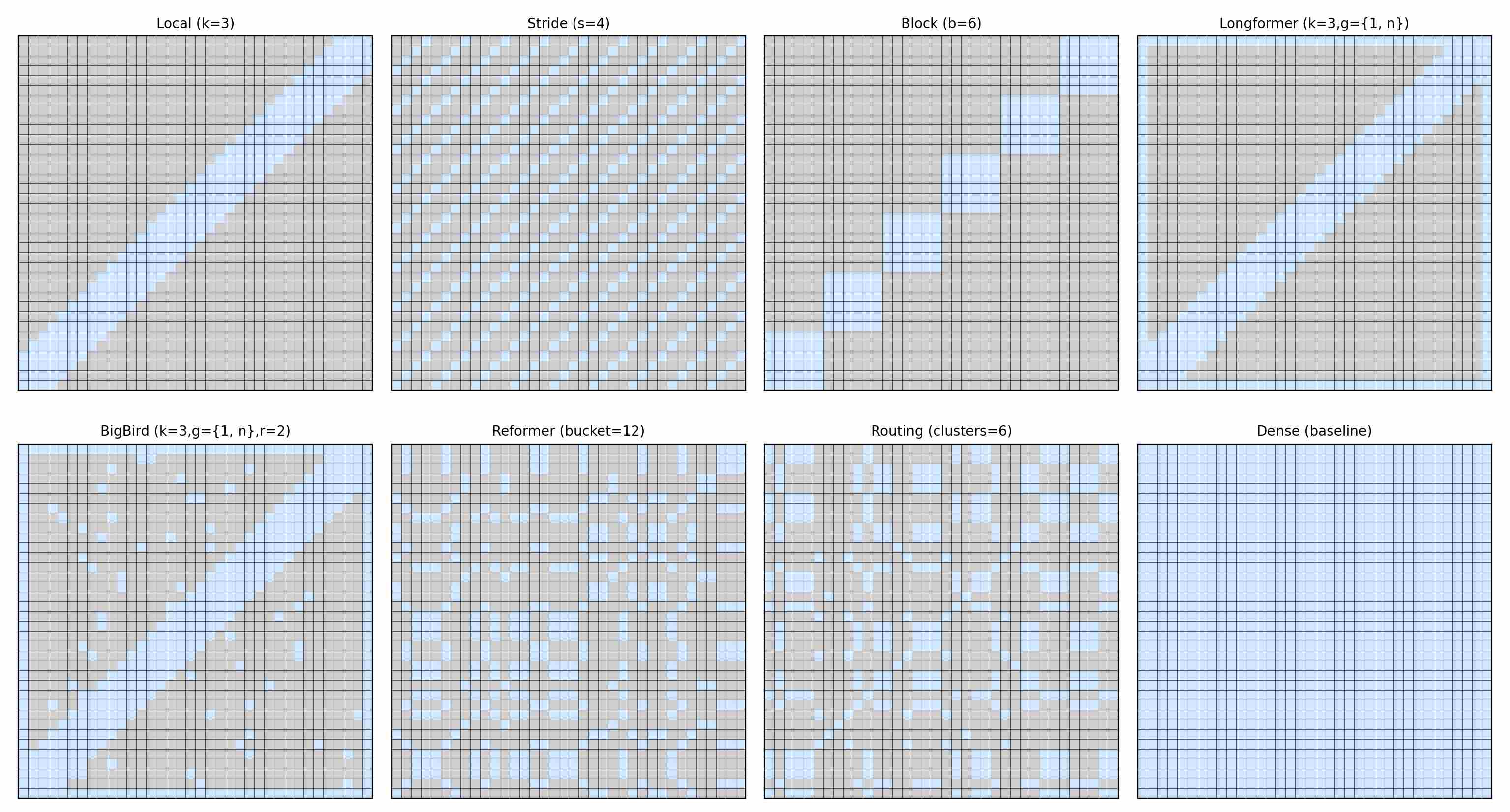
3.2 Sparse & Local Attention
Core Idea: The core assumption is that the most critical information for a given token is often localized or found in a few specific global tokens, rendering a fully dense attention matrix redundant. Instead of computing attention over all $n x n$ pairs, these methods employ predefined sparsity patterns (e.g., sliding windows, dilated/strided windows, global-local attention) to compute only a subset of the attention scores.
Impact: This reduces the complexity from $O(n^2\,d)$ to a more manageable $O(nkd)$, where $k$ is a small, constant factor. This significantly reduces the computational burden during both the forward and backward passes.
Below we summarize the most prominent variants of this families.
Local Attention (Sliding Window) 4: Each query attends only to its neighbors within a fixed window of radius $k$:
\[\mathcal{S}_{\text{local}}(i) = \{ j \;\mid\; |i-j| \leq k \}.\]The time complexity is: $O(nkd)$, and Memory: $O(nk)$.
Stride Attention 10: Queries attend only to keys that share the same position modulo stride $s$:
\[\mathcal{S}_{\text{stride}}(i) = \{ j \;\mid\; j \equiv i \pmod{s} \}.\]Each query sees roughly $n/s$ keys, time complexity is reduced to $O!\left(n\cdot\frac{n}{s}\cdot d\right)$; Memory: $O(n^2/s)$.
Block-Sparse Attention 10: The sequence is partitioned into blocks of size $b$. Queries in block $t$ attend only to keys in the same or neighboring blocks:
\[\mathcal{S}_{\text{block}}(i \in \mathcal{B}_t) = \bigcup_{u=-w}^{w} \mathcal{B}_{t+u}.\]With neighborhood size $w$, each query attends to $(2w+1)b$ keys, Time: $O!\left(n (2w+1) b d\right)$, Memory: $O(n (2w+1) b)$.
Longformer 11: Longformer augments local attention with a small set of global tokens $\mathcal{G}$. Every query attends to its local window plus these global tokens, while global queries themselves attend to the entire sequence:
\[\mathcal{S}_{\text{LF}}(i) = \mathcal{N}_k(i) \cup \mathcal{G}.\]Time complexity is equal to $O(n(k+g)d)$.
BigBird 12: BigBird extends Longformer by adding $r$ random connections:
\[\mathcal{S}_{\text{BB}}(i) = \mathcal{N}_k(i) \cup \mathcal{G} \cup \mathcal{R}_r(i).\]Time complexity is equal to Time: $O(n(k+g+r)d)$.
Reformer 13: Reformer, also known as LSH (Locality-Sensitive Hashing) Attention, replaces the quadratic similarity search with locality-sensitive hashing (LSH). Queries and keys are bucketed via hash codes; attention is restricted to tokens within the same bucket.
With average bucket size $B$, Time: $O(nBd)$. Memory: $O(nB)$.
Routing Transformer 14: The Routing Transformer employs online k-means clustering of queries/keys. Tokens within the same cluster attend to each other, producing structured sparsity:
\[\mathcal{S}_{\text{routing}}(i) = \{ j \;\mid\; \text{cluster}(j)=\text{cluster}(i)\}.\]With cluster size $C$, Time: $O(nCd)$. Memory: $O(nC)$.
We use the following figure to visualize different sparse attentions mechanism. Each heatmap shows the query–key connectivity pattern (blue = attended, gray = masked).
3.3 Linearized Attention
Core Idea: These methods avoid the explicit construction of the matrix $QK^T \in \mathbb{R}^{n\times n}$ by reordering the computation $\text{softmax}(QK^{T}/\sqrt{d})V$. The central thesis of Linearized Attention is to replace the exponential kernel inherent in the softmax function with a general similarity function, $sim(q, k)$, that is decomposable via a kernel feature map $\phi : \mathbb{R}^{d} \to \mathbb{R}^{r}$. Specifically, the similarity is expressed as an inner product in a feature space:
$\text{sim}(q, k) \approx \phi(q) \phi(k)\top$
where
Substituting this kernel into the attention formula, the output for a query $q_i$ becomes:
\[o_i = \sum_{j=1}^{N} \text{sim}(q_i, k_j) v_j = \sum_{j=1}^{N} (\phi(q_i) \phi(k_j)^T) v_j\]By leveraging the associative property of matrix multiplication, the query-dependent term $\phi(q_i)$ can be factored out of the summation:
\[o_i = \phi(q_i)^T \left( \sum_{j=1}^{N} \phi(k_j)^T v_j \right)\]This algebraic manipulation is the cornerstone of all Linearized Attention methods. It fundamentally alters the order of computation from $(Q, K) -> V$ to $(K, V) -> Q$:
Old Order: First, compute the $N \times N$ similarity matrix from $Q$ and $K$, then multiply by $V$. Complexity: $O(N^2 d)$.
New Order: First, compute a “context summary” matrix $\sum_{j=1}^{N} \phi(k_j) v_j^T$ (of size $d_r \times d_v$) from $K$ and $V$. This step has a complexity of $O(N d_r d_v)$. Then, each query $q_i$ attends to this summary. The total complexity becomes linear in $N$ ($O(N d_r d_v)$).
Below, we detail four representative implementations of this principle.
4. FlashAttention: Hardware-Aware Exact Attention
A central challenge of scaling transformers lies not only in the quadratic FLOPs of self-attention but also—more critically—in its quadratic memory footprint and memory traffic. In the conventional implementation, the intermediate attention scores $S=QK^\top/\sqrt{d}$ and probability matrix $P=\mathrm{softmax}(S)$ are both materialized in high-bandwidth memory (HBM), leading to $O(N^2)$ space usage and repeated HBM↔SRAM data transfers. On modern GPUs, where compute throughput vastly outpaces memory bandwidth, this input/output (I/O) overhead becomes the true bottleneck: even though FLOPs scale quadratically, the effective utilization of Tensor Cores can remain as low as 10–20%.
FlashAttention addresses this issue at its root. It does not change the mathematical operator—outputs are bitwise identical to dense softmax attention—but instead reorganizes how computation interacts with hardware. By tiling queries, keys, and values into blocks that fit in on-chip SRAM, and by employing an online (streaming) softmax algorithm that incrementally merges block-level statistics, FlashAttention eliminates the need to store $N^2$ intermediate tensors. As a result, memory complexity drops from quadratic to linear in sequence length, while actual wall-clock time shrinks dramatically due to reduced I/O and higher FLOPs utilization. In essence, FlashAttention demonstrates that exact attention can be made fast by carefully designing the kernel around hardware constraints, rather than by approximating the operator.
In addition to the core symbols, the following symbols will also be used in this chapter
| Category | Symbol / Abbreviation | Definition & Meaning |
|---|---|---|
| 🌀 Streaming Softmax | $B_r$ | Row tile size (blocking size for $Q$) |
| $B_c$ | Column tile size (blocking size for $K,V$) | |
| $i$ | Row index (query index or row in a row tile) | |
| $j$ | Column tile index (key/value tile) | |
| $T_c = \lceil N / B_c \rceil$ | Number of column tiles | |
| $\tilde m_i^{(j)}$ | Row maximum inside tile $j$ | |
| $\tilde \ell_i^{(j)}$ | Row sum of exponentials inside tile $j$ | |
| $\tilde u_i^{(j)}$ | Tile-local unnormalized weighted sum of values | |
| $m_i^{(j)}$ | Global row maximum after tile $j$ | |
| $\ell_i^{(j)}$ | Global row exp-sum after tile $j$ | |
| $\tilde O_i^{(j)}$ | Global unnormalized weighted sum after tile $j$ | |
| $O_i = \tilde O_i^{(T_c)}/\ell_i^{(T_c)}$ | Final normalized row output |
4.1 FlashAttention-V1: I/O-Aware Tiling and Online Softmax
FlashAttention v1 19 is a landmark algorithm designed to accelerate the attention mechanism in Transformers. Its innovation lies not in changing the mathematical output of attention but in fundamentally restructuring its computation to be “I/O-aware,” thereby overcoming the primary performance bottleneck on modern GPUs.
4.1.1 Why Standard Attention is Inefficient on GPUs
To understand FlashAttention v1, one must first understand the GPU memory hierarchy and its performance characteristics. GPUs have two main types of memory:
HBM (High-Bandwidth Memory): This is the large, off-chip GPU memory (e.g., 24GB, 80GB). It has high capacity and bandwidth but is relatively slow to access.
SRAM (Static RAM): This is the small, on-chip cache located next to the GPU’s computing cores. It is extremely fast—orders of magnitude faster than HBM—but has a very limited capacity (a few megabytes).
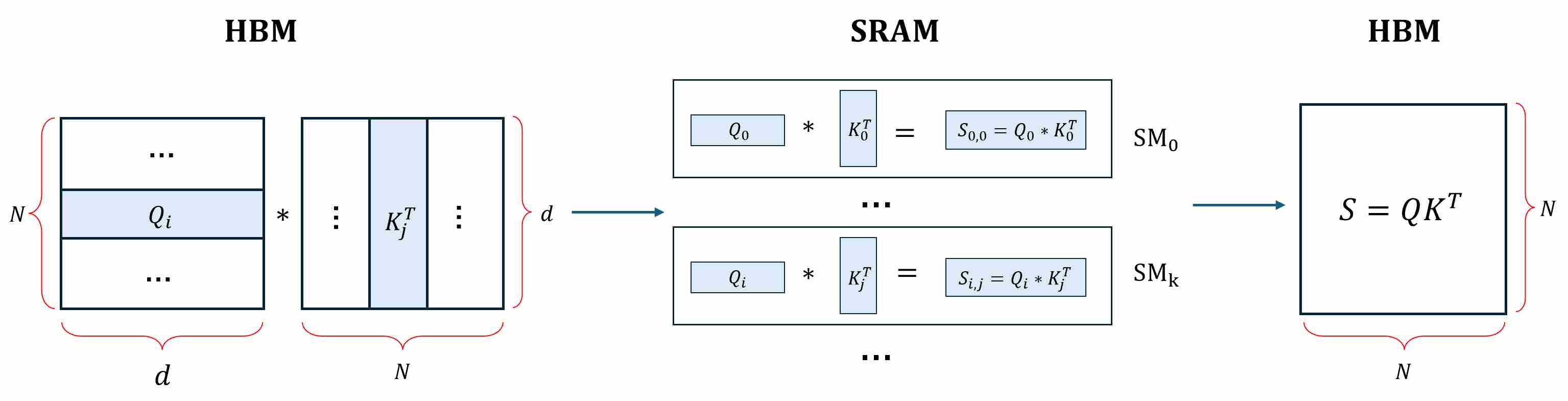
The standard attention computation, $O = \text{softmax}((QK^T))V$ (we ignore the normalization factor $\sqrt{d}$ for convenience), involves several distinct steps that lead to inefficient memory access patterns:
Step 1: Compute and materialize $S = QK^T$. GPUs compute $S$ tile by tile: a small block of $Q$ ($Q_i$) and a small block of $K$ ($K_j$) are loaded into on-chip SRAM (registers/shared memory), a micro-GEMM produces one tile $S_{i,j}=Q_iK^T_j$, and that tile is immediately written to HBM, Repeat until every $S_{i,j}$ has been produced and stored, so that the full matrix $S$ now exists in HBM.
Step 2: Softmax over $S\,(rowwise)$. To compute a numerically stable softmax, the kernel must scan each row to get the rowwise max, then scan again to accumulate. Read tiles of $S$ ($S_i$) from HBM,
\[A_{i, j} = \text{softmax}(S_{i, j}) = \frac{e^{s_{i, j}}}{\sum_{k=1}^{d}{e^{i, k}}} = \frac{e^{s_{i, j}-m_i}}{\sum_{k=1}^{d}{e^{s_{i, k}- m_i}}}\]where $m_i = \max {s_{i,j} (j=1,\dots,N})$. The resulting probabilities are written back to HBM (again tile by tile).
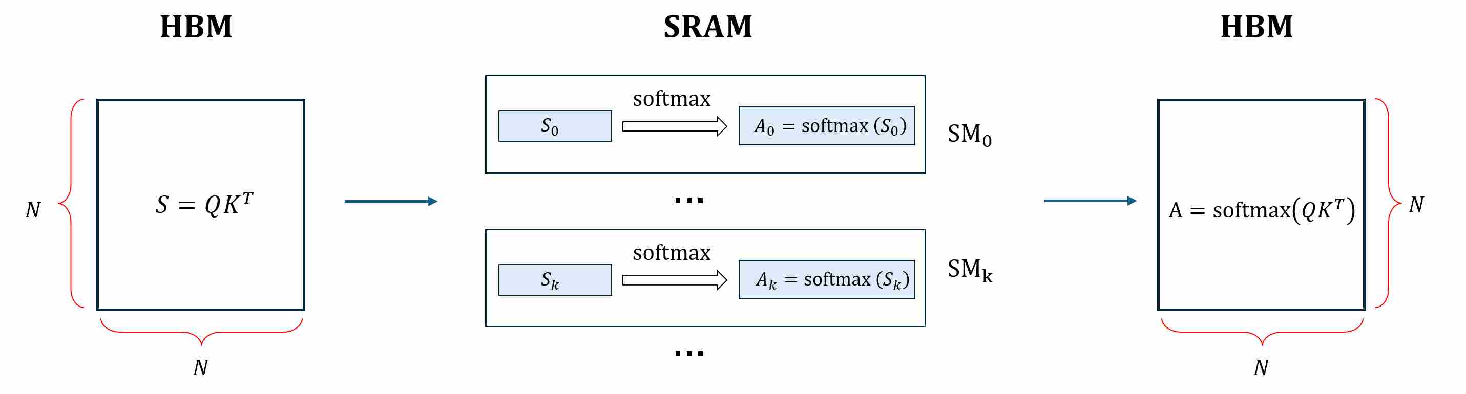
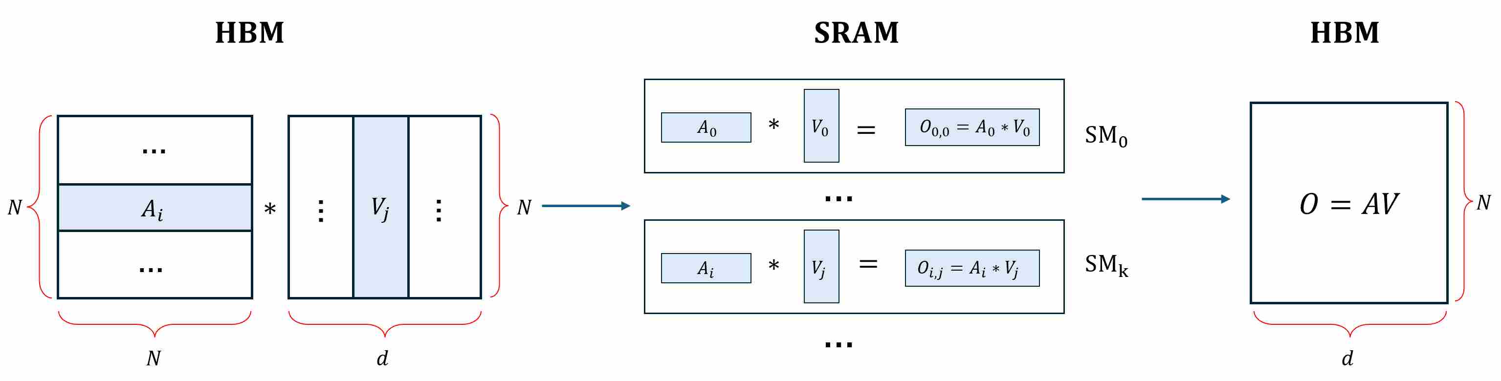
Step 3: Multiply $A$ with $V$ to get output $O$. pull a tile of $A$ ($A_i$) from HBM and a tile of $V$ ($V_j$) from HBM onto the SM, multiply and write it back to HBM. After all tiles are done, accumulate and the full $O$ lives in HBM.
The root problem: The huge $N \times N$ intermediate matrices ($A$ and $S$) are repeatedly read from and written to the slow HBM. When the sequence length $N$ is large (e.g., 8K), this matrix becomes enormous ($8K \times 8K$), and the time spent on memory I/O dwarfs the time spent on actual computation (FLOPs). the dominant cost is I/O, not FLOPs. The kernel sequence is therefore memory-bandwidth bound and forces peak memory to scale as $O(N^2)$.
4.1.2 The Core Idea of FlashAttention-V1
FlashAttention-V1 rethinks attention as an I/O-aware, fused kernel:
Tile the computation so that only small blocks of $Q,K,V$ live in on-chip memory at any time.
Compute and consume scores immediately, via an online (streaming) softmax, so that neither $S$ nor $A$ are ever materialized (saved) in HBM.
Fuse the entire forward pass into a single kernel: $QKᵀ$ -> $\text{softmax}$ -> multiply by $V$ -> accumulate into $O$. This ensures that all intermediate results are kept in fast SRAM without being written back to HBM.
In backward, recompute scores tile-by-tile rather than storing them, while keeping only lightweight per-row statistics.
This preserves the exact semantics of dense attention but achieves I/O-optimality: the minimal possible data movement between HBM and on-chip SRAM, given realistic hardware constraints.
4.1.3 Forward Pass: Tiled, Online Softmax
Let’s focus on computing a single block-row of the output, $O_i$. We partition $K$ and $V$ into $B_c$ column-blocks and $Q$ into $B_r$ row-blocks. The algorithm uses nested loops: an outer loop over blocks of $K$ and $V$ and an inner loop over blocks of $Q$.
Step 1: Partition Q, K, V into tiles
- Split $Q$ with size $N \times d$ into row tiles of size $B_r\times d$.
- Split $K$ and $V$ into column tiles of size $B_c\times d$ and $B_c\times d_v$.
- Assign each row tile of $Q$ to one SM (Streaming Multiprocessor). For example, $\text{SM}_i$ is responsible for all computations related to $Q_i$, this block will remain resident in on-chip memory for the duration of its computation.
Step 2: Stream K & V tiles for computation
For each column tile $j$, Load $K_j$ and $V_j$ from HBM into SMEM/registers, compute local score block $S_{ij}=Q_iK_j^\top$. Within the SM, compute tile-local statistics:
\[\tilde m_i^{(j)}=\max_{k\in j} S_{ik},\quad \tilde \ell_i^{(j)}=\sum_{k\in j} \exp{\left( S_{ik}-\tilde m_i^{(j)} \right)},\quad \tilde u_i^{(j)}=\sum_{k\in j} \exp{\left( S_{ik}-\tilde m_i^{(j)} \right)} V_k\]Update global online softmax statistics (kept per row in registers/SMEM), discard $S_{ij}$ immediately after use—never stored to HBM.
\[\begin{align} m_i^{(j)} &= \max(m_i^{(j-1)}, \tilde m_i^{(j)}), \\[10pt] \ell_i^{(j)} &= \exp{\left( m_i^{(j-1)}-m_i^{(j)} \right)}\ell_i^{(j-1)} + \exp{\left( \tilde m_i^{(j)}-m_i^{(j)} \right)}\tilde \ell_i^{(j)} \end{align}\]After obtaining all the required intermediate results, update the output $O_i$:
\[\begin{align} O_i^j & = \frac{\sum_{k \in {1,\dots,j-1}} \exp{\left( S_{ik}-m_i^{(j)} \right)} V_k + \sum_{k \in {j}} \exp{\left( S_{ik}-m_i^{(j)} \right)} V_k}{l_i^j} \\[10pt] & = \frac{\exp{\left( m_i^{j-1} - m_i^j \right)}\,l_i^{j-1}}{l_i^j}\,O_i^{j-1} + \frac{\exp{\left( \tilde m_i^{(j)} - m_i^j \right)}}{l_i^j}\,\tilde u_i^{(j)} \end{align}\]After all $K/V$ tiles are streamed, Write $O_i$ back to HBM. Only the per-row statistics $(m_i,\ell_i)$ are saved for backward.
This technique is a streaming/parallel version of the log-sum-exp trick. online softmax is an exact computation, identical to dense attention. However, only $Q,K,V,O$ move to/from HBM, $S$ and $A$ are never saved, the peak memory is $O(Nd)$ instead of $O(N^2)$.
4.1.4 Backward Pass: Recomputation Instead of Storage
Computing in blocks and avoiding explicit storage of the large matrix $A$ (or $S$) significantly improves the I/O efficiency of the forward pass, enabling faster computation than the standard approach while maintaining numerical accuracy. However, this also introduces new challenges for backward gradient computation, the backward pass cannot simply reuse $A$, it must reconstruct the relevant probabilities on-the-fly within each tile. This design choice makes the backward algorithm structurally different from the standard one, even though the underlying gradient formulas remain mathematically identical.
| Category | Symbol / Abbreviation | Definition & Meaning |
|---|---|---|
| 📉 Backpropagation | $d_O$ | Gradient of output $O$ |
| $d_A$ | Gradients of $A=\text{softmax}(S)$ | |
| $d_V$ | Gradients of Value $V$ | |
| $d_Q, d_K, d_V$ | Gradients of $Q, K, V$ | |
| $d_S$ | Gradient of score matrix $S$ |
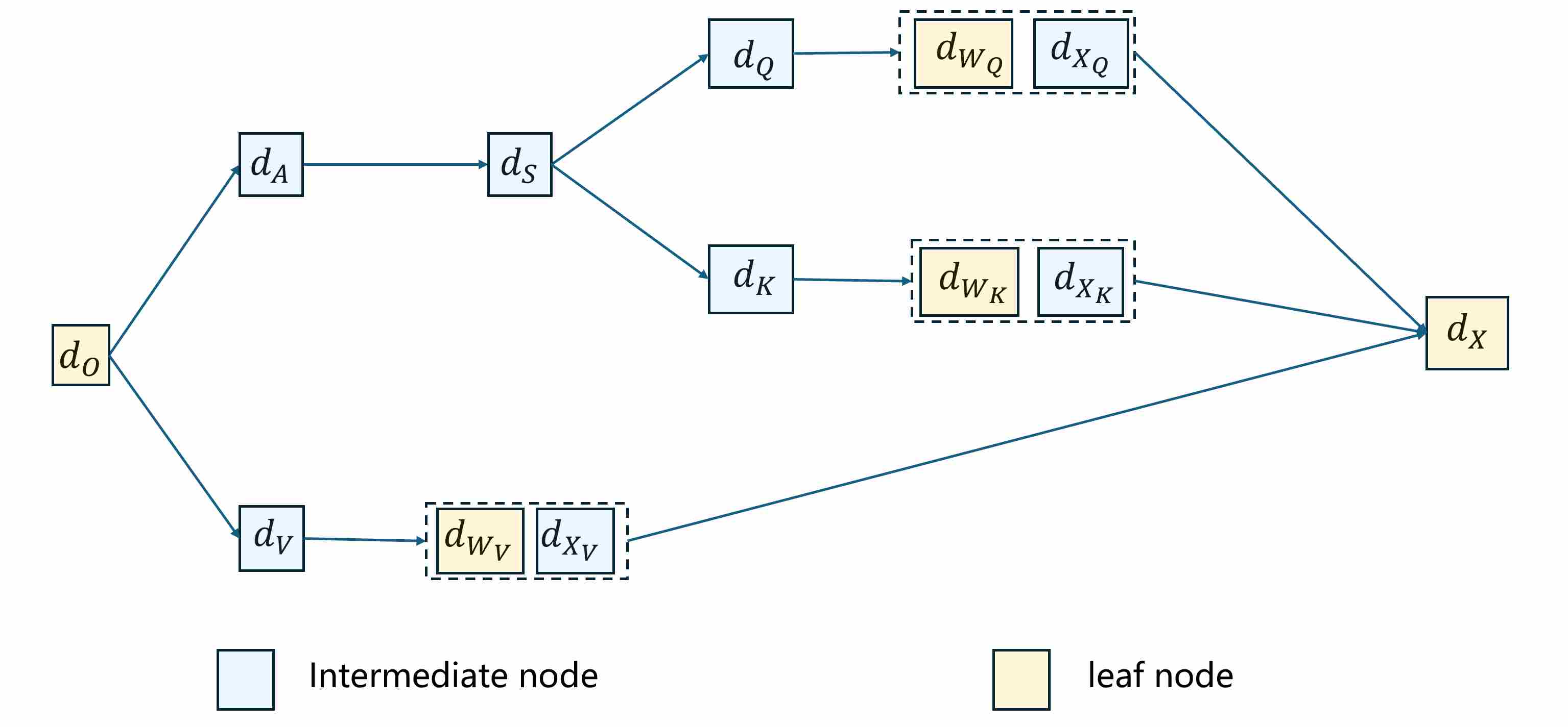
Traditional Gradient Calculation: full backward chain from $d_O$
Let’s brief recap backward propagation of traditional attention. Given the forward attention pass:
\[O = \mathrm{softmax}(\frac{QK^\top}{\sqrt{d}}) V\]The objective is to compute the gradients of the loss function $\mathcal{L}$ with respect to all intermediate and parameter tensors, starting from the upstream gradient $d_O = \partial \mathcal{L}/\partial O$. Gradient flow topology for traditional attention is as follows.
Step 1: Gradients $d_A$ and $d_V$ through the output linear combination. Since $O = A V$, the differentials are governed by standard matrix multiplication rules. The gradients with respect to $V$ and $A$ are
\[d_V = A^\top \cdot d_O,\qquad d_A = d_O \cdot V^\top\]Step 2: Gradients $d_S$ through the softmax function. This is the most intricate step due to the nature of the softmax derivative. Let $ S \in \mathbb{R}^{N \times N} $ be a matrix of input logits. The softmax function is applied row-wise to $S$ to produce the output matrix $A \in \mathbb{R}^{N \times N}$, where each element is given by:
\[A_{ij} = \frac{\exp(S_{ij}-m_i)}{\sum_{k=1}^{N} \exp(S_{ik}-m_i)}.\]Given the upstream gradient $d_A = {\partial L}/{\partial A}$, our goal is to compute the gradient of the loss $ L $ with respect to the input logits $ S $, denoted as $ d_S = {\partial L}/{\partial S} $.
Due to the row-wise application of the softmax, the output $ A_{ij} $ depends only on the elements of the $ i $-th row of $ S $. Therefore, by the chain rule, the gradient for each element $ S_{ij} $ is:
\[d_{S_{ij}} = \frac{\partial L}{\partial S_{ij}} = \sum_{m=1}^{N} \sum_{n=1}^{N} \frac{\partial L}{\partial A_{mn}} \frac{\partial A_{mn}}{\partial S_{ij}} = \sum_{n=1}^{N} \frac{\partial L}{\partial A_{in}} \frac{\partial A_{in}}{\partial S_{ij}}\label{eq:37}\]For each element $A_{in} = \mathrm{softmax}(S_{ij})$, the gradient is
\[\frac{\partial A_{in}}{\partial S_{ij}} = A_{in}\left( \delta_{nj}-A_{ij} \right)\label{eq:38}\]where $\delta_{nj}=1$ when $n=j$, or else $\delta_{nj}=0$. Substitute \ref{eq:38} into \ref{eq:37}, gives
\[\begin{align} d_{S_{ij}} & = \sum_{n=1}^{N} \frac{\partial L}{\partial A_{in}} \frac{\partial A_{in}}{\partial S_{ij}} = \sum_{n=1}^{N} \frac{\partial L}{\partial A_{in}}A_{in}\left( \delta_{nj}-A_{ij} \right) \\[10pt] & = \sum_{n=1}^{N} \frac{\partial L}{\partial A_{in}}A_{in} \delta_{nj} - \sum_{n=1}^{N} \frac{\partial L}{\partial A_{in}} A_{in} A_{ij} \\[10pt] & = \frac{\partial L}{\partial A_{ij}}A_{ij} - A_{ij} \operatorname{rowsum}(d_{A_i} \odot A_i) \\[10pt] & = A_{ij}\left( d_{A_{ij}} - \operatorname{rowsum}(d_{A_i} \odot A_i) \right) \end{align}\]Vectorizing over all rows yields
\[d_S = \bigl(d_A - \operatorname{rowsum}(d_A \odot A)\bigr) \odot A\label{eq:44}\]where $\operatorname{rowsum}(X)$ denotes the vector of row-wise sums, broadcast across columns.
Step 3: Gradients $d_Q$ and $d_K$ through the scaled dot-product scores. The attention scores are defined as $S = \tfrac{1}{\sqrt{d}} Q \cdot K^\top$. Differentiating with respect to $Q$ and $K$ gives
\[d_Q = \frac{1}{\sqrt{d}} d_S \cdot K, \qquad d_K = \frac{1}{\sqrt{d}} d_S^\top \cdot Q.\]Step 4: Gradients through the linear projections. The projections are linear transformations. For $Q = X W_Q$, we obtain
\[d_{W_Q} = X^\top d_Q, \qquad d_{X^{(Q)}} = d_Q W_Q^\top.\]Similarly, for the key and value projections,
\[\begin{align} d_{W_K} = X^\top d_K, \qquad d_{X^{(K)}} = d_K W_K^\top \\[10pt] d_{W_V} = X^\top d_V, \qquad d_{X^{(V)}} = d_V W_V^\top \end{align}\]The total gradient with respect to the input $X$ is the sum of contributions from all three branches:
\[d_X = d_{X^{(Q)}} + d_{X^{(K)}} + d_{X^{(V)}}.\]
Key challenges and Recomputation
From the above analysis, it can be seen that traditional attention backpropagation requires the complete matrix $A$. However, in the forward implementation of FlashAttention v1, we do not save this matrix for memory efficiency. Therefore, during the backward computation in FlashAttention v1, modifications are necessary. The core principle is recomputation.
FlashAttention-V1 avoids materializing $A$ and $S$ in forward. Instead, it saves per-row softmax statistics sufficient to reconstruct probabilities later.
For each row $i$, forward stores
\[m_i = \max_j S_{ij},\qquad \ell_i = \sum_j \exp{\left( S_{ij}-m_i \right)}.\]These are $O(N)$ scalars (often FP32). They suffice to reconstruct matrix $A$ whenever $S_{ij}$ is recomputed.
\[A_{ij} = \frac{\exp{ \left( S_{ij}-m_i \right)}}{\ell_i}\]
Backward Computation in FlashAttention v1
To calculate gradients without matrix $A$. The FlashAttention backward algorithm can be divided into the following three steps.
Step 1: Pre-computation of the \(\mathbf{\text{rowsum}(A \odot {d_A})}\).
The most complex term in the standard backward pass is $d_S$, where
\[{d_S} = A \odot ({d_A} - \text{rowsum}(A \odot {d_A}))\]The FlashAttention algorithm begins with a crucial mathematical insight that simplifies the rowsum term. Let us define a vector $D \in \mathbb{R}^{N}$ where \(D_i = [\text{rowsum}(A_i \odot {d_{A_i}})]\).
Theorem: The vector $D$ can be computed as $D = \text{rowsum}(\text{dO} \odot O)$.
Proof: We aim to prove that for any row $i$: $\text{rowsum}(A_i \odot {d_{A_i}}) = \text{rowsum}(O_i \odot {d_{O_i}})$.
Let’s start with the left-hand side for row $i$:
\[\text{rowsum}(A_i \odot {d_{A_i}}) = \sum_{j=1}^{N} \left( A_{ij} \cdot d_{A_{ij}} \right)\]We substitute the definition $d_A = d_O\,V^T$.
\[\begin{align} \text{rowsum}(A_i \odot {d_{A_i}}) & = \sum_{j=1}^{N} \left( A_{ij} \cdot d_{A_{ij}} \right) = \sum_{j=1}^{N} \left( A_{ij} \sum_{k=1}^{d} ({d_{O_{ik}}} \cdot V_{jk}) \right) \\[10pt] & = \sum_{k=1}^{d} \left( {d_{O_{ik}}} \sum_{j=1}^{N} (A_{ij} \cdot V_{jk}) \right) = \sum_{k=1}^{d} \left( {d_{O_{ik}}} \cdot O_{ik} \right) \\[10pt] & = \text{rowsum}(O_i \odot {d_{O_i}}) \end{align}\]This identity is powerful: it allows us to compute a key component for the $d_S$ bypassing the need for the $O(N^2)$ matrices $A$ and $d_A$. This vector $D$ is computed once at the beginning of the backward pass.
Step 2: accumulate row scalars and $d_V$.
Same as forward process. Backward is organized tile-by-tile over $Q$-row tiles ($B_r$) and $K/V$-column tiles ($B_c$). Assign each row tile of $Q$ to one SM (Streaming Multiprocessor).
Calculate $d_A$ is simple. Load $d_{O_i}$ and $V_j$ from HBM into SRAM, for each block ${\mathbf{d_{A_{ij}}}}$, it can be obtained through dot product.
\[d_{A_{ij}} = d_{O_{ij}} {V_{ij}}^T\]Please note that we do not save ${\mathbf{d_{A_{ij}}}}$. That’s because, like matrix $A$, $d_A$ requires O(N \times N) space memory. Once $d_{A_{ij}}$ is done, we can derive $d_{V_{ij}}$, again tile-by-tile.
\[d_{V_{ij}} = {A_{ij}}^T d_{O_{ij}}\]For ${\mathbf{d_{S_{ij}}}}$, substitute the pre-calculated $D$, $A_{ij}$ and $d_{A_{ij}} into formula \ref{eq:44} to obtain
\[\begin{align} d_{S_{ij}} & = A_{ij}\left( d_{A_{ij}} - \operatorname{rowsum}(d_{A_i} \odot A_i) \right) \\[10pt] & = A_{ij}\left( d_{A_{ij}} - D_i \right) \end{align}\]Once the intermediate gradient $\mathrm{d}_S$ has been formed, the computation of $\mathrm{d}_Q$ and $\mathrm{d}_K$ reduces to a series of dot-product accumulations. Concretely, for each query vector $Q_i$,
\[\mathrm{d}_{Q_i} = \frac{1}{\sqrt d}\sum_{j} \mathrm{d}_{S_{ij}}\,K_j,\]which is a weighted accumulation over the keys $K_j$. Similarly, for each key vector $K_j$,
\[\mathrm{d}_{K_j} = \frac{1}{\sqrt d}\sum_{i} \mathrm{d}_{S_{ij}}\,Q_i.\]Both expressions are dot-product–accumulate operations: each gradient vector is updated by summing products of a scalar coefficient $\mathrm{d}{S{ij}}$ with either a key or a query vector. These operations can be efficiently realized as batched matrix multiplications in practice.
Since the input queries, keys, and values are produced via learned projection matrices,
\[Q = XW_Q,\quad K = XW_K,\quad V = XW_V,\]the gradients must also propagate back to these weights and to the input $X$. Applying the chain rule gives:
\[\mathrm{d}_{W_Q} = X^\top \mathrm{d}_Q, \qquad \mathrm{d}_{W_K} = X^\top \mathrm{d}_K, \qquad \mathrm{d}_{W_V} = X^\top \mathrm{d}_V,\]and the gradient with respect to the input is the accumulated contribution from all three branches:
\[\mathrm{d}_X = \mathrm{d}_Q W_Q^\top + \mathrm{d}_K W_K^\top + \mathrm{d}_V W_V^\top.\]Thus, although FlashAttention v1 employs a tiled recomputation strategy in both the forward and backward passes, the underlying weight and input gradients are obtained through the same linear transformations as in standard attention. The critical difference lies in how $\mathrm{d}_Q, \mathrm{d}_K, \mathrm{d}_V$ are constructed: instead of directly reusing a stored attention matrix, FlashAttention v1 recomputes local probabilities within each tile and forms the gradients by repeated dot-product accumulation.
4.2 FlashAttention-V2: Reducing Non-GEMM Work and Improving Parallelism
FlashAttention-v1 marked a paradigm shift by identifying and solving the I/O bottleneck in standard attention, making the operation compute-bound rather than memory-bound. However, v1 was not the end of the story. Its implementation, while revolutionary, still left significant performance on the table. The primary motivation for FlashAttention-v2 20 was to close this gap, moving from an algorithm that is merely compute-bound to one that is compute-optimal, pushing GPU hardware to its theoretical limits.
FlashAttention-v2 is an engineering tour de force that redesigns the kernel from the ground up to address three subtle but critical limitations in v1: sub-optimal compute utilization, insufficient parallelism on long sequences, and inefficient work partitioning. The result is an algorithm that is up to 2x faster than its predecessor while maintaining the same memory-saving benefits and exactness.
4.3 FlashAttention-V3: Asynchronous Pipelines and FP8 Tensor Cores
5. Memory Efficiency (Leaner)
We have already examined how diffusion model architectures—both U-Net and DiT—can be optimized in terms of computational efficiency and model size. Now we turn to a third, equally important dimension: memory optimization. Memory matters because modern generative models are not only deep but also wide, producing enormous intermediate activations and maintaining billions of parameters. Without careful optimization, training can exceed the physical limits of GPUs, forcing researchers to shrink batch sizes, reduce resolution, or distribute workloads inefficiently. At the same time, inference memory efficiency determines whether these models can run on edge devices or interactive systems, where latency and hardware constraints are strict. Thus, memory optimization is as central to practicality as FLOP reduction or parameter compression.
It is also crucial to distinguish between training and inference when analyzing memory optimizations. The two phases have fundamentally different requirements. During training, memory is dominated by activations and optimizer states: the backward pass requires either storing or recomputing every intermediate tensor, leading to a complexity of
\[M_{\text{train}} = M_{\text{params}} + M_{\text{grads}} + M_{\text{optimizer}} + M_{\text{activations}}.\]By contrast, inference is forward-only and discards gradients and optimizer states:
\[M_{\text{infer}} \approx M_{\text{params}} + M_{\text{activations}}.\]This means techniques like gradient checkpointing or sharded optimizers are relevant only to training, while methods such as quantization, KV caching, and request batching exclusively target inference. Shared techniques, such as mixed precision and FlashAttention, improve both. In practice, this difference explains why training a single Transformer block with naïve attention can balloon to hundreds of gigabytes (due to the $N \times N$ attention matrix), whereas inference can be feasible with only a few gigabytes once efficient attention kernels are used.
Training vs. Inference: Memory & Efficiency Optimizations.
| Category | Technique | Training | Inference | Purpose / Effect |
|---|---|---|---|---|
| Precision & Data Representation | Mixed Precision (FP16/BF16) | ✅ Yes | ✅ Yes | Reduce memory footprint and increase throughput; BF16 avoids loss scaling issues. |
| Quantization (INT8/INT4) | ⚠️ Rare (training instability) | ✅ Yes | Aggressively compress weights/activations for deployment, faster and lighter inference. | |
| Activation / Gradient Handling | Gradient / Activation Checkpointing | ✅ Yes | ❌ No | Reduce activation memory during backpropagation by recomputation. |
| Reversible Layers (RevNet, reversible Transformer) | ✅ Experimental | ❌ No | Reconstruct activations in backward instead of storing them. | |
| Attention Optimizations | FlashAttention / Memory-efficient Attention | ✅ Yes | ✅ Yes | Tile-based attention that avoids storing full $O(N^2)$ matrices; improves speed and memory usage. |
| KV Cache | ❌ No | ✅ Yes (LLMs, AR models) | Cache past key/value pairs to skip recomputation, reducing inference latency. | |
| Optimizer / State Management | 8-bit / 4-bit Optimizers (Adam8bit, Adafactor) | ✅ Yes | ❌ No | Compress optimizer states, greatly reducing memory during training. |
| ZeRO / FSDP / Sharded Optimizer | ✅ Yes | ❌ No | Partition parameters, gradients, and optimizer states across devices to scale training. | |
| Model Structure & Storage | Parameter Sharing / Low-rank Factorization | ✅ Yes | ✅ Yes | Reduce parameter count, making models smaller for both training and inference. |
| Knowledge Distillation | ✅ Yes (train student) | ✅ Yes (deploy student) | Produce smaller, faster student models with comparable accuracy. | |
| System-level Techniques | Gradient Accumulation | ✅ Yes | ❌ No | Simulate larger batch sizes with limited GPU memory. |
| Batching (dynamic batching, flash decoding) | ❌ No | ✅ Yes | Improve throughput by serving multiple inference requests simultaneously. |
5.1 Training-time Memory Efficiency
We’ve made U-Net and DiT faster and smaller; now we make them leaner for training. Diffusion backbones at high resolution create large activations, while optimizers keep sizable state. If left unchecked, you’re forced into tiny batches, unstable training, or cumbersome parallelism. The aim here is to expose the memory budget and the levers that control it—so your computational and parametric gains actually fit on real hardware.
5.1.1 Memory Footprint during the Training Phase
During training, peak memory can be decomposed as
\[M_{\text{train}}=\underbrace{M_{\text{params}}}_{\text{weights}} +\underbrace{M_{\text{grads}}}_{\text{per weight}} +\underbrace{M_{\text{optimizer}}}_{\text{moments & master}} +\underbrace{M_{\text{acts,peak}}}_{\text{activations saved for backward}}.\]Each bucket scales differently and is controlled by different levers.
Model Parameters: $M_{\text{params}}$
What it is. All trainable weights (and a few constant buffers). Linear with parameter size; independent of batch size and resolution.
Levers.
- Precision: FP16/BF16 halves bytes vs. FP32.
- Structure: parameter sharing, low-rank factorization, pruning, distillation.
- Sharding: FSDP / ZeRO-3 shards weights across ranks → each GPU holds a fraction of $M_{\text{params}}$.
Gradients: $M_{\text{grads}}$
What it is. Per-weight gradient tensors resident between backprop and the optimizer step. Same shape as weights; appears after backward; independent of batch size (except via activation footprint that enables the backward).
Levers.
- Precision: half precision grads where stable.
- Sharding: ZeRO-2/3 or FSDP shards grads.
- Step timing: overlapping all-reduce / reduce-scatter with backward can shorten residency (not bytes, but reduces peak concurrency).
Optimizer state: $M_{\text{optimizer}}$
What it is.Per-parameter auxiliary tensors the optimizer maintains to smooth or scale updates (e.g., momentum, first/second moments), plus—under AMP in some setups—a master FP32 copy of the weights. These tensors have the same shape as the parameters and are typically stored in FP32 for numerical stability, so the memory grows linearly with parameter count.
Levers.
- Optimizer choice: 8-bit Adam / Adafactor drastically shrink $m,v$.
- Drop master FP32: where numerically stable (BF16 often is).
- Sharding: ZeRO-1 (states), ZeRO-2 (states+grads), ZeRO-3 (states+grads+params) or FSDP state sharding.
Activations (saved for backward): $M_{\text{acts,peak}}$
What it is. All intermediates you must retain from the forward to compute gradients. This is the only bucket driven by batch size, sequence length, and spatial resolution.
\[M_{activations} \propto \text{Batch Size} \times \text{Input Size} \times \text{Model Depth} \times \text{Hidden Size}\]Levers.
- Activation/gradient checkpointing (rematerialization): store only sparse checkpoint nodes; recompute the rest in backward → activation complexity drops from $O(L)$ to $\sim O(\sqrt{L})$ (even spacing).
- Operator-level kernels: FlashAttention / memory-efficient attention avoids materializing $N^2$ matrices via tiling + online softmax; fused/compiled kernels reduce workspaces.
- Graph design: keep norms/light ops outside checkpoints; in U-Net, checkpoint high-res stages first; in DiT, checkpoint (Attn+MLP) units, more aggressively in early/long-sequence layers.
- Microbatching / gradient accumulation: lower instantaneous activation size without changing the global batch.
5.1.2 Gradient Checkpointing
Deep diffusion models such as U-Nets and DiTs are notoriously memory-hungry during training. The main culprit is not the parameters themselves, but the activations: intermediate tensors that must be stored during the forward pass so that backpropagation can compute gradients. As model depth, resolution, and sequence length increase, the activation footprint quickly outgrows GPU memory capacity, forcing researchers to shrink batch sizes or distribute the model across many devices.
Activation / Gradient Checkpointing was introduced to break this bottleneck. The idea is to trade off additional compute for reduced memory: instead of storing every intermediate tensor, we only store a small set of checkpoint nodes, and recompute the missing activations during the backward pass.
Let a deep network be composed of $L$ modules:
\[h_0 = x, \quad h_i = f_i(h_{i-1}), \quad i=1, \dots, L, \quad y = h_L.\]- Standard training stores all $h_1, h_2, \dots, h_{L-1}$ for use in backpropagation.
- Checkpointing instead selects a sparse subset ${h_{c_1}, h_{c_2}, \dots}$ as checkpoint nodes. During backward pass, when gradients for an intermediate $h_j$ are needed, the network re-executes the forward computations from the nearest checkpoint $h_{c_k}$ up to $h_j$.
Consider a simplified Transformer block as an example.
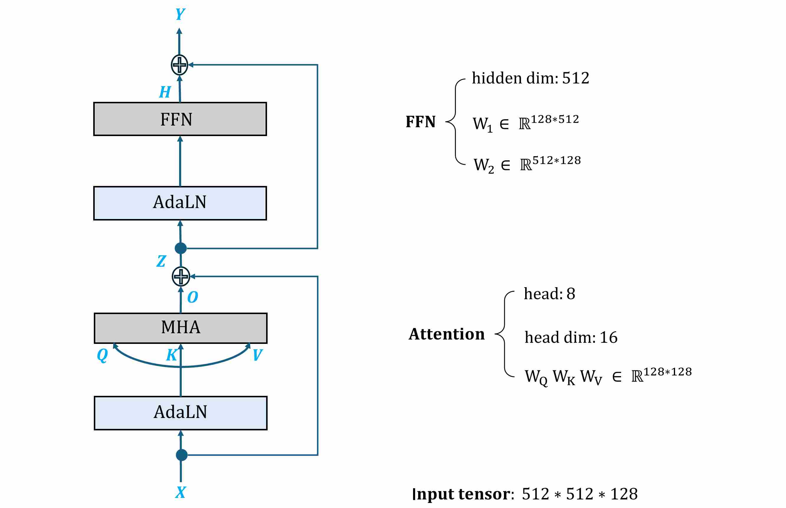
Input tensor: $X \in \mathbb{R}^{512 \times 512 \times 128}$. This can be seen as $N=512 \times 512 = 262{,}144$ tokens, each of dimension $d=128$.
Attention setup: 8 heads, head_dim = 16, with projections $W_Q, W_K, W_V, W_O \in \mathbb{R}^{128 \times 128}$.
FFN setup: hidden size $h=4d=512$, with $W_1 \in \mathbb{R}^{128 \times 512}$, $W_2 \in \mathbb{R}^{512 \times 128}$.
Precision: FP32 (4 bytes per element).
Case A: Naive Attention (store $A$ or $S$), No Checkpointing
Activations: include $X,Q,K,V,O,Z,H,Y$, plus the full attention score or probability matrix:
\[S = QK^\top \in \mathbb{R}^{N \times N}, \quad A = \text{softmax}(S).\]Memory:
- Each $N \times d$ tensor ($X, Q,K,V,O,Y$): $262{,}144 \times 128 \times 4 \approx 0.125$ GiB.
- Each $N \times h$ tensor ($Z,H$): $262{,}144 \times 512 \times 4 \approx 0.500$ GiB.
- $A$ or $S$: $N^2 = 6.87\times10^{10}$ elements $\Rightarrow$ 256 GiB.
Peak activation memory ≈ 257.75 GiB (if only $A$ or $S$ is stored), or ≈ 513 GiB if both are stored.
Case B: Memory-Efficient Attention (no materialized $A/S$), No Checkpointing
Activations: include $X,Q,K,V,O,Z,H,Y$. Use an “online softmax” or tiling scheme as in FlashAttention to avoid store $A$ and $S$.
Memory:
$$ tensors ($X,Q,K,V,O,Y$) of shape $N \times d$ → 0.75 GiB.
$2$ tensors of shape $N \times h$ → 1.00 GiB.
Peak activation memory ≈ 1.75 GiB.
Case C: Case B + Block-Level Gradient Checkpointing
Activations: Only checkpoint the block input $X$ and output $Y$; everything else is recomputed in backward.
Memory:
- $2$ tensors ($X,Y$) of shape $N \times d$ → 0.25 GiB.
Peak activation memory ≈ 0.25 GiB., but requires recomputing $Q,K,V,O,Z,H$ during backward pass.
5.1.3 Sharded Training via ZeRO Redundancy Optimizer
While gradient checkpointing tackles the dynamic memory costs associated with activations, the static memory footprint—comprising model parameters, gradients, and optimizer states—remains a major bottleneck.
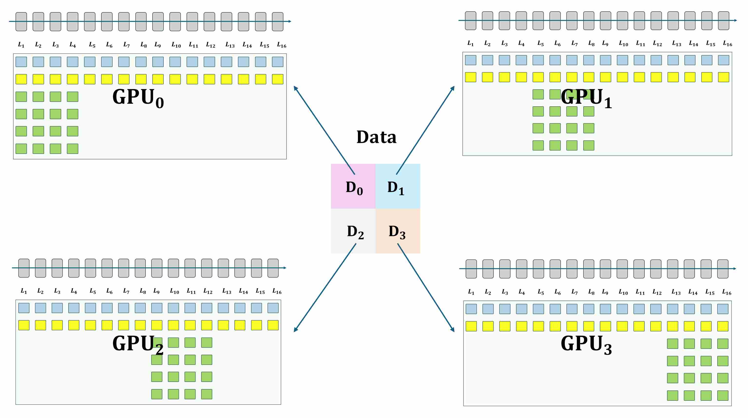
Consider the example in the figure below: suppose we are training a 16-layer network. At the start of training, all necessary data must be stored in GPU high-bandwidth memory (HBM), including model parameters, gradients, optimizer states, and activations. This already creates a heavy memory footprint on a single device.
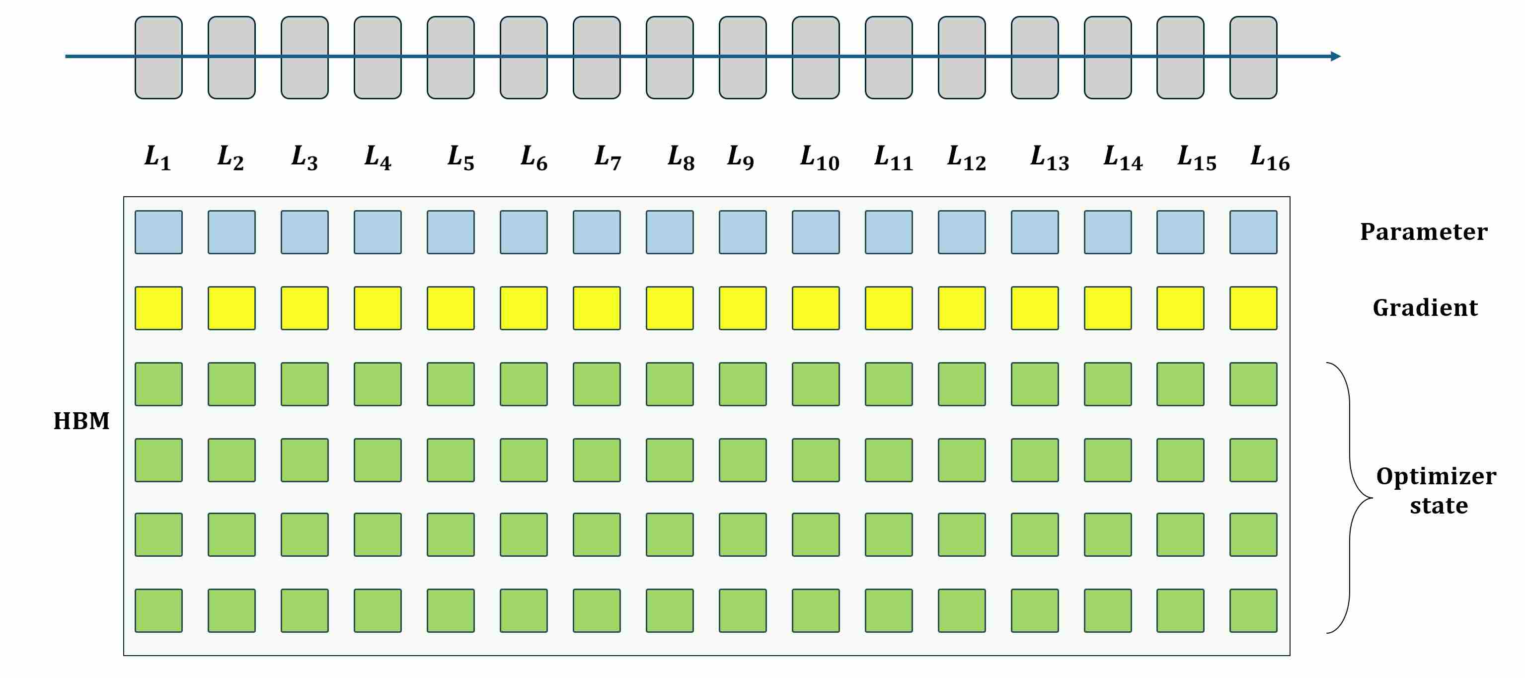
When scaling to large models, training on a single GPU is no longer feasible, and we typically employ Distributed Data Parallel (DDP) to accelerate training across multiple GPUs. In DDP, each GPU holds a full copy of the model and performs local forward/backward passes, while gradients are averaged across devices to keep parameters synchronized. Although this design is simple and effective for parallelism, it introduces a critical drawback: every GPU redundantly stores the entire set of parameters, gradients, and optimizer states.
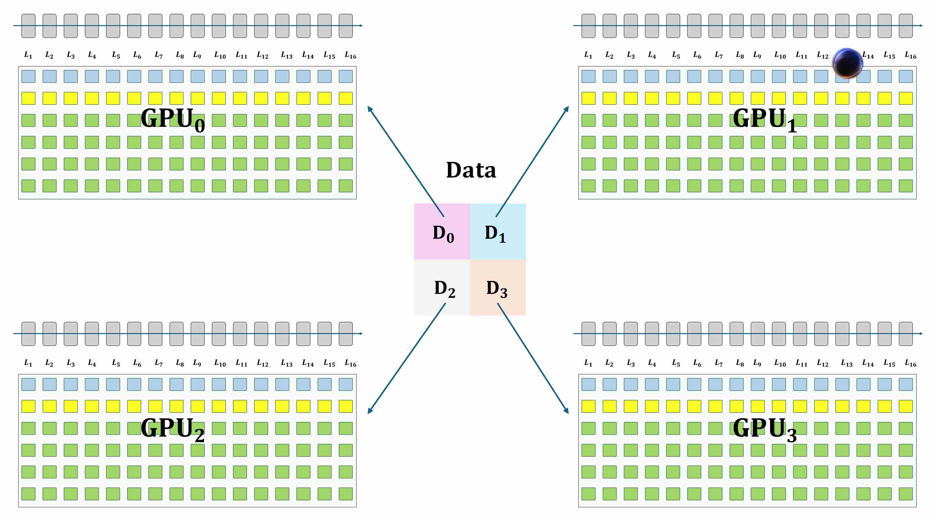
For small models this overhead is tolerable, but for diffusion backbones with billions of parameters it becomes prohibitive, exhausting memory long before compute is saturated.
This limitation is the main motivation for the ZeRO Redundancy Optimizer (ZeRO), ZeRO addresses this issue by eliminating unnecessary replication. Instead of storing the entire set of parameters, gradients, and optimizer states on each GPU, ZeRO partitions them across devices, so that each GPU holds only a shard. Through this sharding strategy, memory scales linearly with the number of GPUs, enabling the training of models that would otherwise be impossible under conventional DDP.
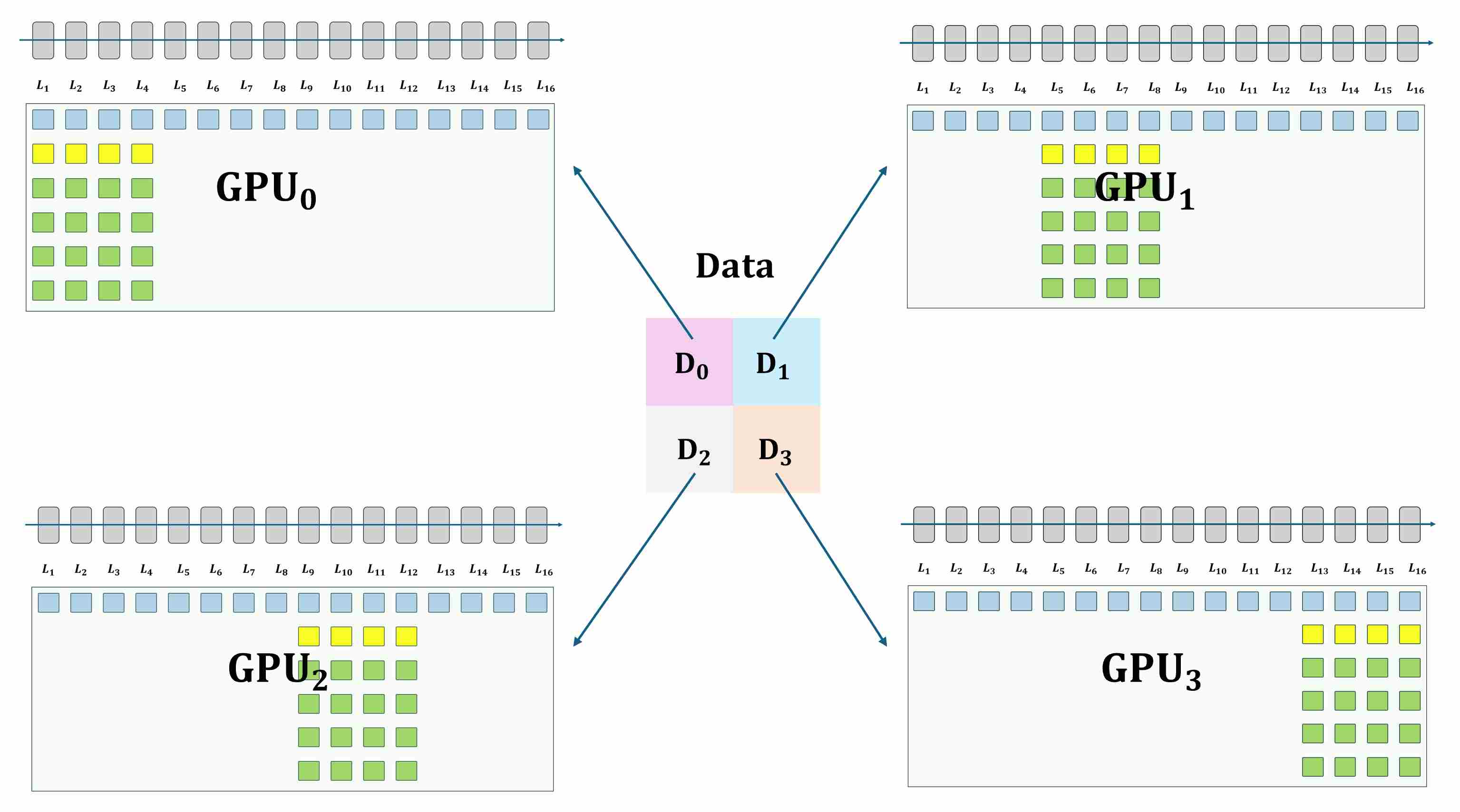
ZeRO-Stage 1: Partitioning Optimizer States
The first and largest source of redundancy is typically the optimizer state. For an optimizer like AdamW, this includes two moments (momentum and variance) for every model parameter, often stored in full FP32 precision. This can easily be 2-3 times the size of the model parameters themselves.
- Mechanism: ZeRO-1 shards only the optimizer states. Each GPU is responsible for updating only its assigned partition of the model’s parameters.
Process: After gradients are synchronized via a standard AllReduce (just like in DDP), each GPU performs its optimizer step on its local shard of parameters. An
AllGatheroperation then ensures all GPUs receive the fully updated parameters for the next forward pass.Benefit: Drastically reduces memory by distributing the largest component of static memory. Memory per GPU can be reduced to:
\[\tfrac{1}{N}M_{\text{optimizer}} + M_{\text{params}} + M_{\text{grads}}\]
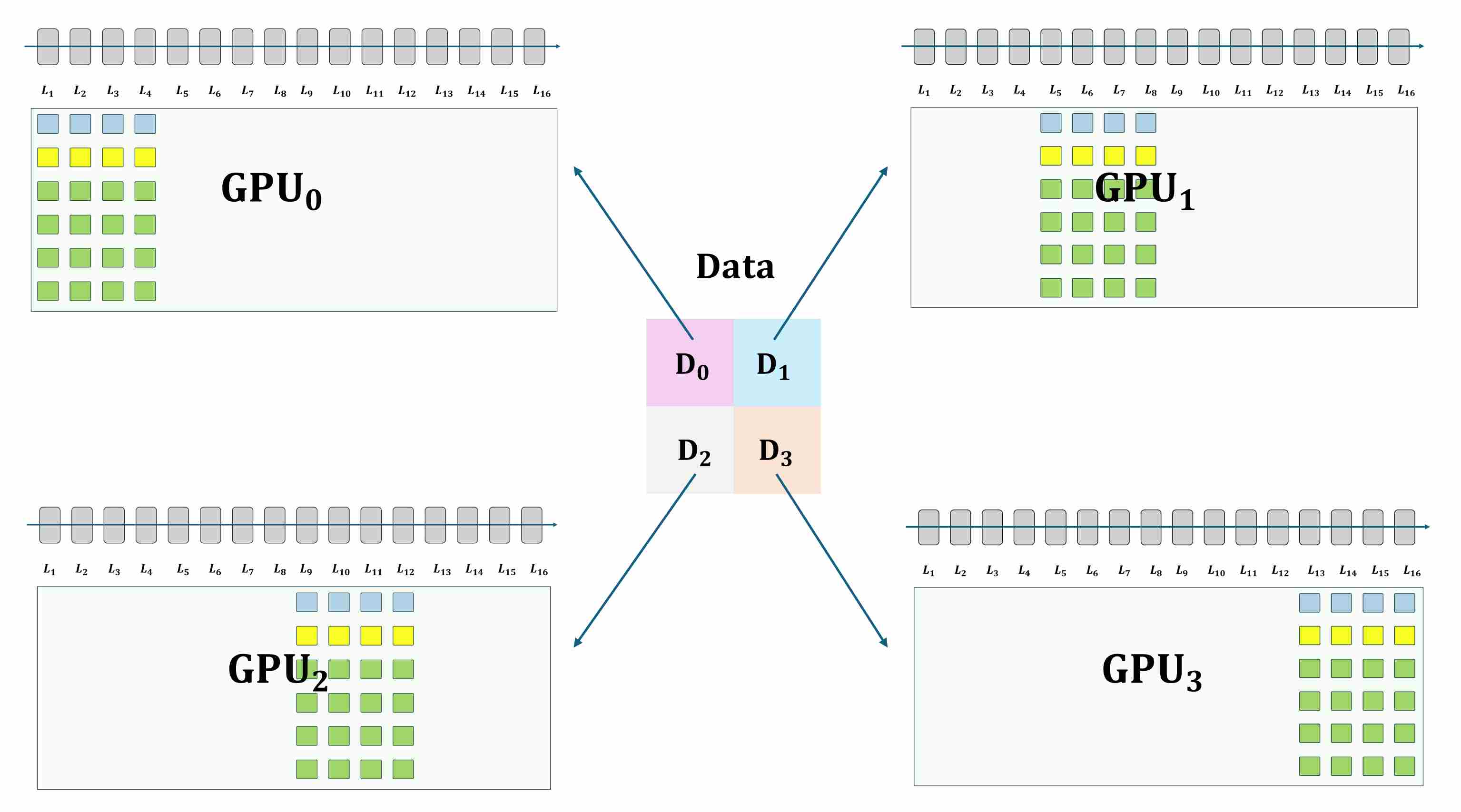
ZeRO-Stage 2: Partitioning Gradients and Optimizer States
Stage 2 builds on Stage 1 by also eliminating gradient redundancy. In DDP, after backpropagation, each GPU holds a full copy of the gradients before they are averaged.
- Mechanism: In addition to optimizer states, gradients are also sharded. Instead of an
AllReduce, aReduceScatteroperation is used during backpropagation. This operation both computes the sum and distributes the result, so each GPU ends up with only the gradient partition it needs for its update. - Process: The
ReduceScatterefficiently delivers the correct gradient slice to the GPU responsible for that parameter shard. The subsequent parameter update andAllGatherare similar to Stage 1. - Benefit: Saves additional memory equivalent to the size of the model’s parameters.
ZeRO-Stage 3: Partitioning Parameters, Gradients, and Optimizer States
This is the most powerful stage, enabling the training of truly enormous models. ZeRO-3 extends sharding to the model parameters themselves.
- Mechanism: Each GPU only holds a 1/N slice of the parameters, gradients, and optimizer states at all times.
- Process: During the forward and backward passes, as the computation proceeds from one layer to the next, the required parameters for that specific layer are dynamically materialized on all GPUs via an
AllGatheroperation. Once the layer’s computation is complete, the non-owned parameters are immediately discarded. - Benefit: The memory footprint per GPU is reduced to a fraction of the full model size, theoretically allowing for the training of models of near-infinite size, limited only by the memory required to hold a single layer’s parameters and activations. PyTorch’s native implementation, FSDP (Fully Sharded Data Parallelism), is largely based on the principles of ZeRO-3.
5.2 Inference-time Memory Efficiency
5.1.2 Memory Footprint during the Inference Phase
9. References
Rombach R, Blattmann A, Lorenz D, et al. High-resolution image synthesis with latent diffusion models[C]//Proceedings of the IEEE/CVF conference on computer vision and pattern recognition. 2022: 10684-10695. ↩
Saharia C, Chan W, Saxena S, et al. Photorealistic text-to-image diffusion models with deep language understanding[J]. Advances in neural information processing systems, 2022, 35: 36479-36494. ↩
Podell D, English Z, Lacey K, et al. Sdxl: Improving latent diffusion models for high-resolution image synthesis[J]. arXiv preprint arXiv:2307.01952, 2023. ↩
Liu Z, Lin Y, Cao Y, et al. Swin transformer: Hierarchical vision transformer using shifted windows[C]//Proceedings of the IEEE/CVF international conference on computer vision. 2021: 10012-10022. ↩ ↩2
Chollet F. Xception: Deep learning with depthwise separable convolutions[C]//Proceedings of the IEEE conference on computer vision and pattern recognition. 2017: 1251-1258. ↩
Howard A G, Zhu M, Chen B, et al. Mobilenets: Efficient convolutional neural networks for mobile vision applications[J]. arXiv preprint arXiv:1704.04861, 2017. ↩
He K, Zhang X, Ren S, et al. Deep residual learning for image recognition[C]//Proceedings of the IEEE conference on computer vision and pattern recognition. 2016: 770-778. ↩
Sandler M, Howard A, Zhu M, et al. Mobilenetv2: Inverted residuals and linear bottlenecks[C]//Proceedings of the IEEE conference on computer vision and pattern recognition. 2018: 4510-4520. ↩
Tan M, Le Q. Efficientnet: Rethinking model scaling for convolutional neural networks[C]//International conference on machine learning. PMLR, 2019: 6105-6114. ↩
Child R, Gray S, Radford A, et al. Generating long sequences with sparse transformers[J]. arXiv preprint arXiv:1904.10509, 2019. ↩ ↩2
Beltagy I, Peters M E, Cohan A. Longformer: The long-document transformer[J]. arXiv preprint arXiv:2004.05150, 2020. ↩
Zaheer M, Guruganesh G, Dubey K A, et al. Big bird: Transformers for longer sequences[J]. Advances in neural information processing systems, 2020, 33: 17283-17297. ↩
Kitaev N, Kaiser Ł, Levskaya A. Reformer: The efficient transformer[J]. arXiv preprint arXiv:2001.04451, 2020. ↩
Roy A, Saffar M, Vaswani A, et al. Efficient content-based sparse attention with routing transformers[J]. Transactions of the Association for Computational Linguistics, 2021, 9: 53-68. ↩
Shen Z, Zhang M, Zhao H, et al. Efficient attention: Attention with linear complexities[C]//Proceedings of the IEEE/CVF winter conference on applications of computer vision. 2021: 3531-3539. ↩
Katharopoulos A, Vyas A, Pappas N, et al. Transformers are rnns: Fast autoregressive transformers with linear attention[C]//International conference on machine learning. PMLR, 2020: 5156-5165. ↩
Choromanski K, Likhosherstov V, Dohan D, et al. Rethinking attention with performers[J]. arXiv preprint arXiv:2009.14794, 2020. ↩
Peng H, Pappas N, Yogatama D, et al. Random feature attention[J]. arXiv preprint arXiv:2103.02143, 2021. ↩
Dao T, Fu D, Ermon S, et al. Flashattention: Fast and memory-efficient exact attention with io-awareness[J]. Advances in neural information processing systems, 2022, 35: 16344-16359. ↩
Dao T. Flashattention-2: Faster attention with better parallelism and work partitioning[J]. arXiv preprint arXiv:2307.08691, 2023. ↩