
Analysis of the Stability of Diffusion Model Training
Published:
📚 Table of Contents
Diffusion models have achieved unprecedented success in the field of generative modeling, producing incredibly high-fidelity images, audio, and other data. However, the training process of these models presents several unique challenges like divergence, vanishing gradients, or unstable training behavior during the learning process. A stable training process ensures that the model produces good quality samples and converges efficiently over time without suffering from numerical instabilities.
In previous post, we review the basic concepts of diffusion model, this post we will focus on training.
Brief recap
For generative models, we expect our model $p_{\theta}$ (parameterized by $\theta$) to be as close as possible to the true distribution $p_{data}$. Based on the KL divergence, we derive that
\[\mathbb{KL}(p_{data}(x) \parallel p_{\theta}(x)) = \int p_{data}(x)\log (p_{data}(x))dx - \int p_{data}(x)\log(p_{\theta}(x))dx\label{eq:1}\]The first term, $\int p_{data}(x) \log (p_{data}(x))dx$, is the entropy of the true distribution $p_{data}$, it is a constant with respect to the model parameters $\theta$. The second term, $\int p_{data}(x)\log(p_{\theta}(x))dx$, is the expected log-likelihood of the model under the true distribution. Thus, minimizing KL divergence is equal to maximize log-likelihood $p_{\theta}(x)$, where $x \sim p_{data}$.
From Maximum likelihood to ELBO
Let $x_0$ be the original image, and $x_i (i=1,2,…,T)$ be the image with noise added to $x_0$. We wish to maximise
\[\log p_{\theta}(x_0)=\log \int p_{\theta}(x_{0:T}) dx_{1:T} \label{eq:2}\]Introduce the forward process $q(x_{1:T} \mid x_0)$ (a Markov chain with fixed noise‑schedule). Using Jensen’s inequality gives the evidence lower bound:
\[\begin{align} \log p_\theta(x_0) \geq \mathcal{L}_\text{ELBO} & = \mathbb{E}_q \left[ \log p_\theta(x_0 \mid x_1) - \log \frac{q(x_{T} \mid x_0)}{p_\theta(x_{T})} - \sum_{t=2}^T \log \frac{q(x_{t-1} \mid x_t, x_0)}{p_\theta(x_{t-1} \mid x_t)} \right]\label{eq:3} \end{align}\]The first term is reconstruction loss, the second term is prior matching, both of them are extremely small and can be ignored. Therefore, what we are truly concerned about is the third item, which also known as denoising term.
From KL collapses to a mean MSE
For each denoising step, both forward posterior $q(x_{t-1} \mid x_t, x_0) \sim \mathcal{N}(\mu_{q}, \sigma_{q}^2I)$ and backward posterior $p_{\theta}(x_{t-1} \mid x_t) \sim \mathcal{N}(\mu_{\theta}, \sigma_{\theta}^2I)$ are gaussian distributions. For two Gaussians with identical covariance, if we fix the two variances are equal to $\sigma_{q}^2$, then the KL divergence is equal to:
\[\mathbb{KL}\left(q(x_{t-1} \mid x_t, x_0) \parallel p_{\theta}(x_{t-1} \mid x_t) \right) = \frac{1}{2\sigma_q^2} \|{\mu}_{q} - \mu_{\theta}(x_t, t)\|_2^2 + \text{const}\label{eq:4}\]Hence, for each denoising step, the loss function equals to
\[\mathcal{L}_{\text{denoise}} = \mathbb{E}_q \left[ \|\mu_q - \mu_{\theta}(x_t, t)\|^2 \right]\label{eq:5}\]$\mu_q$ is the true target we want to predict, How do we calculate the value of $\mu_q$? Let’s first decompose forward posterior $q(x_{t-1} \mid x_t, x_0)$ :
\[q(x_{t-1} \mid x_t, x_0)=\frac{q(x_{t} \mid x_{t-1})q(x_{t-1} \mid x_{0})}{q(x_{t} \mid x_{0})} \propto q(x_{t} \mid x_{t-1})q(x_{t-1} \mid x_{0})\label{eq:6}\]where
\[q(x_{t} \mid x_{t-1}) \sim \mathcal{N}(x_{t-1};\mu_1, \sigma_1^2I),\ \ \mu_1=\frac{1}{\sqrt{\alpha_t}}x_{t},\ \ \sigma_1^2=\frac{1-\alpha_t}{\alpha_t} \\[10pt] q(x_{t-1} \mid x_{0}) \sim \mathcal{N}(x_{t-1};\mu_2, \sigma_2^2I), \ \ \mu_2=\sqrt{\bar \alpha_{t-1}}x_{0},\ \ \sigma_2^2=1-\bar \alpha_{t-1}\label{eq:7}\]The product of two Gaussian distributions is itself a Gaussian distribution,
\[\mu_{q} = \frac{\mu_1\sigma_2^2+\mu_2\sigma_1^2}{\sigma_1^2+\sigma_2^2} = \frac{\sqrt{\alpha_t}(1 - \bar{\alpha}_{t-1}) x_t + \sqrt{\bar{\alpha}_{t-1}} (1 - \alpha_t) {x}_0}{1 - \bar{\alpha}_t}\label{eq:8}\]Combining equations \ref{eq:5} and \ref{eq:8}, Our goal is to construct a neural network $\mu_{\theta}$, which takes $x_t$ and $t$ as inputs, such that the output of the network is as close as possible to $\mu_q$.
Re-parameterising the mean with different target predictor
Following equation \ref{eq:8}, we can dirrectly build a network $\mu_{\theta}$ to output $\mu_{q}$. However, in practice, we usually do not directly fit the value of $\mu_{q}$, mainly due to the following reasons.
$\mu_{q}$ is an affine function of $x_t$, which is known at training and test time, there is no need for the network to “reproduce” it. If we regress $\mu_{q}$ directly, the network wastes capacity relearning a large known term and must also learn the residual that actually depends on the unknown clean content.
The mean target value is highly time-dependent scaling across $t$, which means that the output of the network is unstable, it is usually extremely difficult for a network to output results with a large variance range.
Instead of asking the network to output $\mu_{q}$ directly, the community typically uses four common prediction targets to train diffusion models: $\epsilon$-prediction, $x_0$-prediction, $v$-prediction, score-prediction. If we regard the original image $x_0$ and noise $\epsilon$ as two orthogonal dimensions, then All the common targets are linear in $(x_0, \epsilon)$
$x_0$-prediction (aka sample-prediction in Diffusers)
In $x_0$-prediction, the neural network is trained to directly estimate the clean original data $x_0$ from the noisy input $x_t$ at timestep $t$. Denoted the network as $ x_{\theta}(x_t, t)$, and the predicted output is \(\hat{x}_0\), this approach reparameterizes the predicted mean $\mu_{\theta}$ using the estimated \(\hat{x}_0\). Substituting into Equation \ref{eq:8}, the mean becomes:
\[\mu_{\theta}(x_t, t) = \frac{\sqrt{\alpha_t}(1 - \bar{\alpha}_{t-1}) x_t + \sqrt{\bar{\alpha}_{t-1}} (1 - \alpha_t) \hat{x}_0}{1 - \bar{\alpha}_t}\label{eq:9}\]The loss function then simplifies to minimizing the MSE between the true $x_0$ and the predicted $\hat{x}_0$:
\[\mathcal{L} = \mathbb{E}_{x_0, t, \epsilon} \left[ \| x_0 - x_{\theta}(x_t, t) \|^2 \right]\label{eq:10}\]Pros
This parameterization is advantageous because the target $x_0$ has a consistent scale across timesteps, reducing the variance in network outputs and improving training stability.
Cons
The primary drawback of $x_0$-prediction lies in the uneven learning difficulty across signal-to-noise ratio (SNR) regimes, which induces heterogeneous gradient behaviors and ultimately hinders training convergence.
$\epsilon$-prediction
The $\epsilon$-prediction paradigm tasks the network with predicting the noise $\epsilon$ added during the forward process. This parameterization leverages the forward noising equation to express the clean data $x_0$ in terms of the noise $\epsilon$ via a simple linear transformation (equation \ref{eq:11}).
\[x_t = \sqrt{\bar{\alpha}_t} x_0 + \sqrt{1 - \bar{\alpha}_t} \epsilon \ \Longrightarrow \ x_0=\frac{x_t-\sqrt{1 - \bar{\alpha}_t} \epsilon}{\sqrt{\bar{\alpha}_t}}\label{eq:11}\]Substituting this reparameterized form of $x_0$ (with $\hat{\epsilon}$ in place of $\epsilon$) into Equation \ref{eq:8} for the mean gives:
\[\mu_{\theta}(x_t, t) = \frac{1}{\sqrt{\alpha_t}} \left( x_t - \frac{1 - \alpha_t}{\sqrt{1 - \bar{\alpha}_t}} \hat{\epsilon} \right)\label{eq:12}\]The loss function then simplifies to minimizing the MSE between the true noise $\epsilon$ and the predicted $\hat{\epsilon}$:
\[\mathcal{L} = \mathbb{E}_{x_0, t, \epsilon} \left[ \| \epsilon - \epsilon_{\theta}(x_t, t) \|^2 \right]\label{eq:13}\]Pros
This parameterization is advantageous because the target $\epsilon$ is timestep-independent target distribution since $\epsilon \sim \mathcal{N}(0, I)$.
Cons
Like $x_0$-prediction, $\epsilon$-prediction also suffers from the uneven learning difficulty problems, which needs re-weighting $ w(t) $ to promote balanced learning across the noise spectrum. We will conduct more in-depth analysis in the following sections.
$v$-prediction
Velocity ($v$)-prediction combines elements of both $x_0$ and $\epsilon$ predictions by forecasting a velocity term $v$ that interpolates between them. Defined velocity as \(v = \sqrt{\bar{\alpha}_t} \epsilon - \sqrt{1 - \bar{\alpha}_t} x_0\) (or its normalized variant), the network predicts \(\hat{v} = v_{\theta}(x_t, t)\). The mean $\mu_{\theta}$ can be expressed in terms of \(\hat{v}\):
\[\mu_{\theta}(x_t, t) = \sqrt{\alpha_t}x_t- \frac{(1-\alpha_t)\sqrt{\bar \alpha_{t-1}}}{\sqrt{1-\bar \alpha_t}}{\hat v}\label{eq:14}\]The loss function then simplifies to minimizing the MSE between the true velocity $v$ and the predicted \(\hat{v}\):
\[\mathcal{L} = \mathbb{E}_{x_0, t, \epsilon} \left[ \| v - v_{\theta}(x_t, t) \|^2 \right]\label{eq:15}\]This hybrid approach adapts dynamically to timestep: in high SNR regimes, it behaves like $\epsilon$-prediction, while in low SNR regimes, it resembles $x_0$-prediction. This adaptability enhances stability by balancing gradient flows across SNR levels, reducing divergence risks, but requires precise calibration of the velocity formulation to avoid numerical instabilities during backpropagation.
Score-prediction
This parameterization draws from the score-based generative modeling framework, where the neural network estimates the score function $s_{\theta}(x_t, t) = \nabla_{x_t} \log p_t(x_t)$, representing the gradient of the log-probability density at the noisy state $x_t$. In Gaussian diffusion models, the score is directly related to the noise via \(s(x_t, t) = -\frac{\epsilon}{\sqrt{1 - \bar \alpha_t}}\), allowing a re-expression of the noise $\epsilon$ in terms of the score. Starting from the forward noising equation and substituting the equivalent form \(\epsilon = -\sqrt{1 - \bar{\alpha}_t} \, s(x_t, t)\), the predicted mean \(\mu_{\theta}\) is derived by inserting this into Equation \ref{eq:8}:
\[\mu_{\theta}(x_t, t) = \frac{1}{\sqrt{\alpha_t}} \left( x_t + (1 - \alpha_t) \, s_{\theta}(x_t, t) \right)\]The loss function simplifies to minimizing the MSE between the true score $s(x_t, t)$ and the predicted \(\hat{s} = s_{\theta}(x_t, t)\):
\[\mathcal{L} = \mathbb{E}_{x_0, t, \epsilon} \left[ \| s(x_t, t) - s_{\theta}(x_t, t) \|^2 \right]\]Pros Integrated in models like Score-Based Generative Models (SGMs) and aligned with continuous-time formulations, this approach facilitates theoretical connections to stochastic differential equations (SDEs) and enhances generalization across noise schedules.
Cons However, it may introduce scaling sensitivities in discrete timesteps, potentially leading to instabilities if the score magnitudes are not properly normalized, necessitating adaptive weighting or variance adjustments during training. In general, it has more theoretical value but is rarely used in practice.
Imbalances in Learning Across Timesteps and SNR Regimes
Diffusion training looks deceptively simple: draw a noisy pair $(x_0, x_t)$ from the forward process and regress a target $y$ with an MSE. Although the four targets — $\epsilon$-prediction, $x_0$-prediction, $v$-prediction, and score-prediction — are linearly transformable, in practice, which target you regress matters—a lot. Different targets place learning pressure on different SNR bands, change the numerical conditioning of the regression, and interact differently with weighting/preconditioning and the sampler you’ll use at test time. This section builds a unified, quantitative picture of why these differences arise and how to correct them.
They exhibit uneven learning difficulty under unit weights $w(t)\equiv 1$. Using SNR rather than the raw timestep $t$ reveals these imbalances clearly.
A unifying lens: the $(x_0,\epsilon)$ basis and SNR
Forward noising:
\[x_t \;=\; a\,x_0 + b\,\epsilon, \quad \epsilon\sim\mathcal N(0,I).\]Where in DDPM, $a=\sqrt{\bar\alpha_t},\; b=\sqrt{1-\bar\alpha_t}$. $Define the signal-to-noise ratio (SNR):
\[\mathrm{SNR}(t)\;=\;\frac{a^2}{b^2}\;=\;\frac{\bar\alpha_t}{1-\bar\alpha_t}\]- High SNR $\Rightarrow$ early timesteps (signal-dominated; easier).
- Low SNR $\Rightarrow$ late timesteps (noise-dominated; harder).
Any target used in practice is a linear functional of $(x_0,\epsilon)$. The common four are
- $\epsilon$-prediction: $y_t=\epsilon$
- $x_0$-prediction: $y_t=x_0$
- $v$-prediction: $y_t=v := a\,\epsilon - b\,x_0$ (an orthogonalized combo)
- score-prediction: $y_t=s(x_t,t)= -\dfrac{x_t-a x_0}{b^2}= -\dfrac{\epsilon}{b}$ (conditional score of $q(x_t|x_0)$)
They are linearly equivalent (you can recover one from another), but that does not mean they have the same learning dynamics under the same loss and weights.
Root Causes of Differences (Unified View: Correlation → Conditional Expectation → Gradient)
It is well established that the four common training targets in diffusion models — $\epsilon$-prediction, $x_0$-prediction, $v$-prediction, and score-prediction — can all be expressed under a unified mean-squared error (MSE) loss formulation:
\[\ell(\theta; x_t, y) = \|\, y - f_{\theta}(x_t, t) \,\|^2 \quad \Longrightarrow \quad \mathcal{L} = \mathbb{E} \left[ \ell(\theta; x_t, y\right]\label{eq:20}\]where $y$ is the chosen target, and $f_{\theta}(x_t, t)$ is the model output given $x_t$ and timestep $t$. Although these targets are linearly interconvertible, empirical results show substantial differences in training dynamics and final performance depending on the target choice.
The MSE loss can be decomposed using the standard bias-variance decomposition for regression. Treating this as predicting $ y $ given $ x_t $, the total loss is:
\[\mathcal{L} = \mathbb{E}_{x_t} \left[ \mathbb{E}_{y \mid x_t} \left[ \left\| y - f_\theta(x_t, t) \right\|^2 \right] \right]\]Expanding the inner expectation:
\[\mathbb{E}_{y \mid x_t} \left[ \left\| y - f_\theta \right\|^2 \right] = \mathbb{E}_{y \mid x_t} \left[ \left\| (y - \mu) + (\mu - f_\theta) \right\|^2 \right] = \operatorname{Var}(y \mid x_t) + \left\| \mu - f_\theta \right\|^2\]where $ \mu = \mathbb{E}[y \mid x_t] $, and the cross term vanishes because $ \mathbb{E}_{y \mid x_t} [y - \mu] = 0 $. Thus:
\[\mathcal{L} = \underbrace{\mathbb{E}_{x_t} \left[ \operatorname{Var}(y \mid x_t) \right]}_{\text{Irreducible noise (unlearnable)}} + \underbrace{\mathbb{E}_{x_t} \left[ \left\| \mathbb{E}[y \mid x_t] - f_\theta(x_t, t) \right\|^2 \right]}_{\text{Learnable part}}\]Irreducible noise part: This is the inherent variance of $ y $ given $ x_t $, which depends on the data distribution and diffusion process. Even a perfect model (where $ f_\theta = \mathbb{E}[y \mid x_t] $) cannot reduce the loss below this value.
Learnable part: This measures how well $ f_\theta $ approximates the optimal predictor $ \mathbb{E}[y \mid x_t] $, which can be minimized to zero through training.
1) Correlation: Measuring Task Difficulty
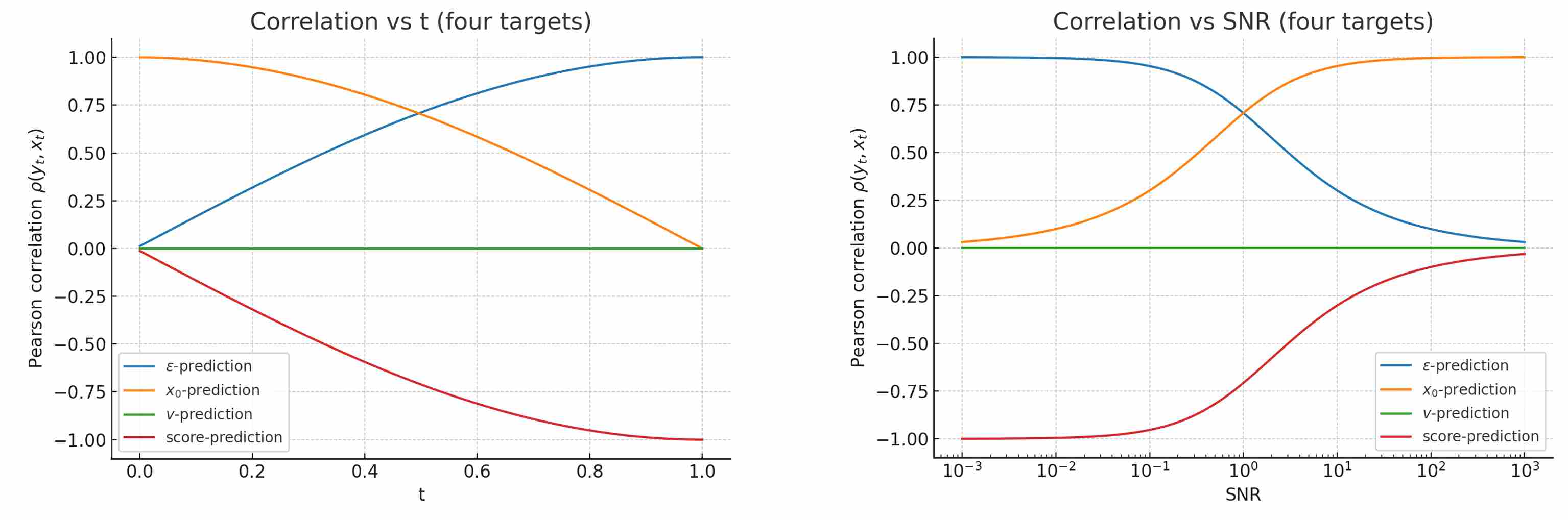
For a target $y$ (which can be $\epsilon$, $x_0$, $v$, or $s=\nabla_{x_t} \log p_t$), we compute its Pearson correlation with $x_t$ at different SNR levels:
\[\rho_t = \dfrac{\mathrm{Cov}(y,x_t)}{\sqrt{\mathrm{Var}(y)\mathrm{Var}(x_t)}}\]A higher correlation implies that $y_t$ can be well approximated as a linear function of $x_t$, making the prediction task easier.
- $\epsilon$-prediction: $\rho_{\epsilon, x_t} = \dfrac{1}{\sqrt{1+\mathrm{SNR}}}$ — strong at low SNR, weak at high SNR, easiest to learn in low-SNR regions but harder in high-SNR regions.
- $x_0$-prediction: $\rho_{x_0, x_t} = \sqrt{\dfrac{\mathrm{SNR}}{1+\mathrm{SNR}}}$ — strong at high SNR, weak at low SNR, easiest to learn in high-SNR regions but harder in low-SNR regions.
- $v$-prediction: $\rho_{v, x_t} = 0$ — orthogonal to $x_t$ for all SNR, tends to maintain a more balanced correlation across SNR, indicating more uniform difficulty.
- score-prediction: $\rho_{s, x_t} = -\dfrac{1}{\sqrt{1+\mathrm{SNR}}}$ — same magnitude as $\epsilon$ but opposite sign.
The following figure shows Pearson correlation between four target values and $x_t$, with the horizontal axis corresponding to SNR and T respectively.
2) Conditional Expectation: Measuring Optimization Signal Strength
A fundamental principle of statistics states that to minimize the loss function (equation \ref{eq:20}), the optimal model $f_{\theta}^{\star}$ must predict the conditional expectation of the target y given the input $x_t$, i,e.,
\[f_{\theta}^{\star} = \mathbb{E}(y \mid x_t)\]To understand why one target $y$ is better than another, we must analyze the properties of its conditional mean.
We start from the forward diffusion process equation: $x_t = a_t x_0 + b_t \epsilon$, taking the conditional expectation with respect to $ x_t $ on both sides (noting that $ E(x_t | x_t) = x_t $, and using linearity of expectation):
\[E(x_t | x_t) = a_t E(x_0 | x_t) + b_t E(\epsilon | x_t)\ \ \Longrightarrow \ \ x_t = a_t E(x_0 | x_t) + b_t E(\epsilon | x_t)\]Since $ x_t $ is observed, the above equality holds deterministically, Linking All Targets via $ \mathbb{E}[\epsilon \mid x_t] $:
$ \epsilon $-prediction: \(\mathbb{E}[\epsilon \mid x_t] \quad \text{(direct target)}\)
$ x_0 $-prediction:
\[\mathbb{E}[x_0 \mid x_t] = \frac{x_t - b_t \mathbb{E}[\epsilon \mid x_t]}{a_t} \quad \Longrightarrow \quad \mathbb{E}[x_0 \mid x_t] = \frac{x_t}{a_t} - \frac{b_t}{a_t} \mathbb{E}[\epsilon \mid x_t]\]$ v $-prediction: With $ v = a_t \epsilon - b_t x_0 $, substituting the above conditional means yields:
\[\begin{align} & \mathbb{E}[v \mid x_t] = a_t \, \mathbb{E}[\epsilon \mid x_t] - b_t \, \mathbb{E}[x_0 \mid x_t] \\[10pt]\Longrightarrow \quad & \mathbb{E}[v \mid x_t] = a_t \, \mathbb{E}[\epsilon \mid x_t] - b_t \, \left( \frac{x_t}{a_t} - \frac{b_t}{a_t} \mathbb{E}[\epsilon \mid x_t] \right) \\[10pt] \Longrightarrow \quad & \mathbb{E}[v \mid x_t] = -\frac{b_t}{a_t} x_t + \frac{1}{a_t} \mathbb{E}[\epsilon \mid x_t] \end{align}\]Score-prediction: in the Gaussian forward process, the score function is defined as
\[s(x_t, t) = \nabla_{x_t} \log p(x_t \mid t) \quad \Longrightarrow \quad s=-\frac{x_t-a_t \, x_0}{b_t^2}\]Taking the conditional expectation with respect to $ x_t $ on both sides:
\[\begin{align} & \mathbb{E}[s \mid x_t] = -\frac{x_t-a_t \, \mathbb{E}[x_0 \mid x_t]}{b_t^2} \\[10pt] \Longrightarrow \quad & \mathbb{E}[s \mid x_t] = -\frac{\mathbb{E}[\epsilon \mid x_t]}{b_t} \end{align}\]
It can be observed that the conditional expectation of all targets can be expressed as a linear combination of $x_t$ and $\mathbb{E}[\epsilon \mid x_t]$.
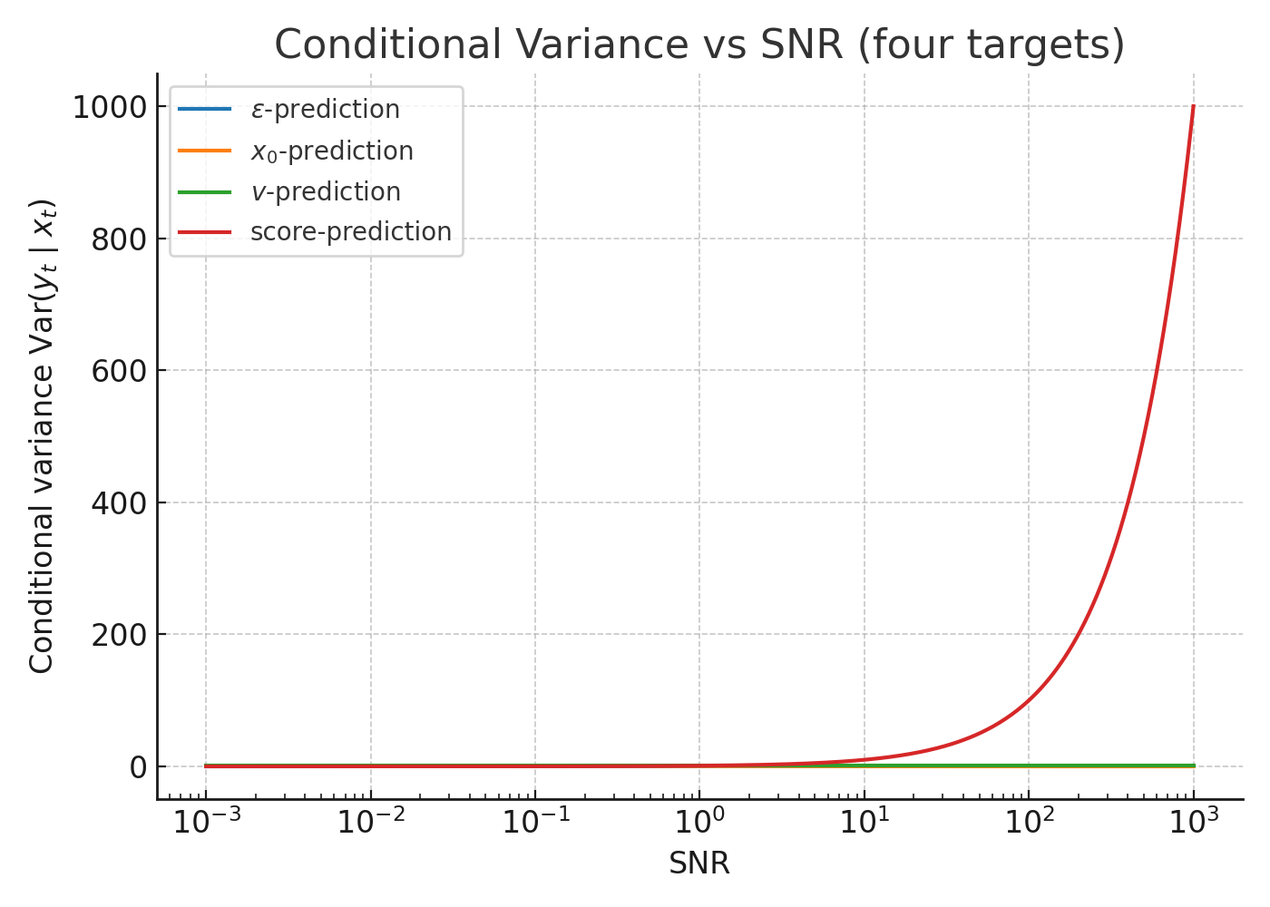
3) Conditional Variance: Linking to Gradient Energy
Near the optimum, the sample gradient of the MSE loss is $2(\hat{y}_t - y_t)$.
With $\hat{y}_t \approx \mathbb{E}[y_t \mid x_t]$, the gradient variance is dominated by the irreducible noise: \(\mathbb{E}\,\|\nabla_\theta \mathcal{L}_t\|^2 \;\propto\; \mathrm{Var}(y_t \mid x_t).\)
Per target:
- $\epsilon$: $\dfrac{\mathrm{SNR}}{1+\mathrm{SNR}}$
- $x_0$: $\dfrac{1}{1+\mathrm{SNR}}$
- $v$: $1$
- score: $\mathrm{SNR}$
Implications without any re-weighting:
- $\epsilon$: large gradient energy at high SNR, small at low SNR.
- $x_0$: the opposite trend.
- $v$: equal gradient energy across SNR.
- score: gradient energy grows with SNR, potentially unstable in high-SNR regimes.
Figure 3: Conditional variance vs SNR (four targets)
Summary
Learning imbalance arises from two factors:
1) how predictability ($\rho$, $k_y$) varies across SNR, and
2) how noise-driven gradient energy $\mathrm{Var}(y_t \mid x_t)$ is distributed over timesteps.
SNR-aware weighting strategies (e.g., P2, min-SNR, EDM) directly reshape these profiles, yielding more stable and efficient training.
2. Multi-Metric Comparison under Unit Weights
Let $a=\sqrt{\bar\alpha_t}$, $b=\sqrt{1-\bar\alpha_t}$, so $\mathrm{SNR}=\dfrac{a^2}{b^2}$ and $x_t=a\,x_0+b\,\epsilon$. We consider four targets:
- $\epsilon$-prediction;
- $x_0$-prediction;
- $v=a\,\epsilon-b\,x_0$;
- score $s(x_t,t)=-\dfrac{x_t-a\,x_0}{1-a^2}=-\dfrac{\epsilon}{b}$.
2.1 Metrics, Formulas, and Rationale
| Metric | Definition | Why it Matters |
|---|---|---|
| Correlation $\rho(y_t,x_t)$ | $\dfrac{\mathrm{Cov}(y_t,x_t)}{\sqrt{\mathrm{Var}(y_t)\mathrm{Var}(x_t)}}$ | Linear predictability; $\rho^2$ equals $R^2$. |
| Bayes Error | $\mathrm{Var}(y_t\mid x_t)$ | Irreducible noise of the regression target. |
| Gradient Scale $G$ | $\propto \sqrt{\mathrm{Var}(y_t\mid x_t)}$ | Proxy for SGD magnitude per SNR. |
| Mutual Information | $-\tfrac12\log(1-\rho^2)$ | Info-theoretic predictability (nats). |
| Predictability Ratio $\Pi$ | $\dfrac{\mathrm{Var}(\mathbb E[y_t\mid x_t])}{\mathrm{Var}(y_t\mid x_t)}$ | Signal-to-noise ratio of the target. |
| Bayes Slope $k_y$ | $\mathrm{Cov}(y_t,x_t)$ | Gain of the Bayes regressor; matters for conditioning. |
| Unconditional Var | $\mathrm{Var}(y_t)$ | Target scale (can destabilize training if large). |
| Preconditioning Factor $g_y$ | $1/\sqrt{\mathrm{Var}(y_t\mid x_t)}$ | Output scaling that flattens gradient scale. |
2.2 Closed-Form Results (Unit Weights)
- Correlation:
- $\epsilon$: $\rho=\dfrac{1}{\sqrt{1+\mathrm{SNR}}}$;
- $x_0$: $\rho=\sqrt{\dfrac{\mathrm{SNR}}{1+\mathrm{SNR}}}$;
- $v$: $\rho=0$;
- score: $\rho=-\dfrac{1}{\sqrt{1+\mathrm{SNR}}}$.
- Bayes Error $\mathrm{Var}(y\mid x_t)$:
- $\epsilon$: $\dfrac{\mathrm{SNR}}{1+\mathrm{SNR}}$;
- $x_0$: $\dfrac{1}{1+\mathrm{SNR}}$;
- $v$: $1$;
- score: $\mathrm{SNR}$.
- Gradient Scale $G\propto \sqrt{\mathrm{Var}(y\mid x_t)}$:
- $\epsilon$: $\sqrt{\dfrac{\mathrm{SNR}}{1+\mathrm{SNR}}}$;
- $x_0$: $\dfrac{1}{\sqrt{1+\mathrm{SNR}}}$;
- $v$: $1$ (flat);
- score: $\sqrt{\mathrm{SNR}}$.
- Mutual Information (nats):
- $\epsilon$: $\tfrac12\log(1+\tfrac{1}{\mathrm{SNR}})$;
- $x_0$: $\tfrac12\log(1+\mathrm{SNR})$;
- $v$: $0$;
- score: same as $\epsilon$.
- Predictability Ratio $\Pi$:
- $\epsilon$: $\tfrac{1}{\mathrm{SNR}}$;
- $x_0$: $\mathrm{SNR}$;
- $v$: $0$;
- score: $\tfrac{1}{\mathrm{SNR}}$.
- Bayes Slope $k_y$:
- $\epsilon$: $\dfrac{1}{\sqrt{1+\mathrm{SNR}}}$;
- $x_0$: $\sqrt{\dfrac{\mathrm{SNR}}{1+\mathrm{SNR}}}$;
- $v$: $0$;
- score: $-1$.
- Unconditional Var $\mathrm{Var}(y)$:
- $\epsilon$: $1$; $x_0$: $1$; $v$: $1$; score: $1+\mathrm{SNR}$.
- Preconditioning $g_y\propto 1/\sqrt{\mathrm{Var}(y\mid x_t)}$:
- $\epsilon$: $\sqrt{\dfrac{1+\mathrm{SNR}}{\mathrm{SNR}}}$;
- $x_0$: $\sqrt{1+\mathrm{SNR}}$;
- $v$: $1$;
- score: $\mathrm{SNR}^{-1/2}$.
Baseline curves(unit weights)
(这些图已在上一小节给出,路径请按你仓库替换)
- Correlation vs SNR:
.../correlation_vs_snr.png - Gradient scale vs SNR:
.../gradscale_vs_snr.png - Predictability Ratio:
.../predictability_ratio_vs_snr.png - Mutual Information:
.../mutual_information_vs_snr.png - Bayes Error:
.../bayes_error_vs_snr.png - Bayes Slope:
.../bayes_regressor_slope_vs_snr.png - Target Variance:
.../target_variance_vs_snr.png - Preconditioning Factor:
.../preconditioning_vs_snr.png
3. SOTA Weighting & Preconditioning: What They Do and How They Look
We summarize practical SOTA schemes and visualize before vs after on key targets using the gradient-scale proxy (the metric most immediately affected by weighting/target scaling).
注:相关性与 Bayes error 由数据生成过程决定,不随损失权重改变;因此主要比较梯度尺度的再分配效果。
3.1 p2-weighting (perception-prioritized)
A common form: \(w_{\mathrm{p2}}(t)\propto (\mathrm{SNR}(t)+c)^{-\gamma},\;\; \gamma>0,\; c\in[0,1].\)
- 作用:抑制高 SNR(早期)步的梯度,补偿中/低 SNR。
- 推荐:搭配 $\epsilon$-prediction。
epsilon: unit vs p2(示例参数 $\gamma!=!1,\,c!=!1$)

3.2 Min-SNR weighting / clipping
给 $\mathrm{SNR}$ 设置下限 $\tau$ 形成权重(常见实现等价于在低 SNR 放大损失): \(\tilde{\mathrm{SNR}}(t)=\max(\mathrm{SNR}(t),\tau),\quad w_{\min\text{-}SNR}(t)\approx \frac{\tilde{\mathrm{SNR}}(t)}{\mathrm{SNR}(t)}.\)
- 作用:防止低 SNR 区域梯度“饿死”,改善末期还原质量。
- 推荐:常配合 $x_0$-prediction 或 $v$-prediction。
x0: unit vs min-SNR(示例 $\tau!=!10^{-1}$)

3.3 EDM-style preconditioning
在噪声水平 $\sigma^2=(1-\bar\alpha_t)/\bar\alpha_t=1/\mathrm{SNR}$ 空间做输入/输出预条件和权重(典型例:$w(\sigma)!\propto!1/(\sigma^2!+!1)$),核心目标是让有效梯度在 $\log\sigma$ 轴上趋于均匀。
- 作用:通过目标缩放与输入标准化,近似实现 $g_y\cdot G(\mathrm{SNR})\approx \text{const}$。
- 推荐:对 $\epsilon$ 与 $x_0$ 尤其有效;对 $v$ 变化很小(其本就较平坦)。
epsilon: unit vs EDM 预条件(示意以 $g_\epsilon$ 实现)

x0: unit vs EDM 预条件(示意以 $g_{x_0}$ 实现)

score: unit vs EDM 预条件(示意以 $g_{s}$ 实现)

v: unit vs EDM 预条件(几乎无变化)

3.4 Loss-aware / difficulty-aware weighting
根据近期损失大小或梯度方差动态调整 $w(t)$(如 $w!\leftarrow!1/\mathrm{EMA}[\mathcal L_t]$ 或按 SNR 分桶估计方差后反比缩放)。
- 作用:自适应聚焦“未学好”的时间段,兼容任意目标。
- 注意:需防止过度振荡,引入平滑与上/下界。
4. Practical Reading
- $\epsilon$-prediction:原生偏向高 SNR;用 p2/EDM 拉平。
- $x_0$-prediction:原生偏向低 SNR;用 min-SNR/EDM 补齐高 SNR。
- $v$-prediction:梯度近乎平坦;通常只需轻量预条件或直接用 unit weights。
- score-prediction:尺度随 SNR 增长快;需强预条件与/或上界控制。
Bottom line. Multi-metric, SNR-indexed analysis shows where each target is imbalanced under unit weights and how modern reweighting/预条件 reshape gradient energy to be more uniform — improving stability and convergence speed without changing expressivity.