
Analysis of the Stability and Efficiency of Diffusion Model Training
📅 Published: | 🔄 Updated:
📘 TABLE OF CONTENTS
- Part I — Foundation and Preliminary
- Part II — Analyze the causes of training instability and inefficiency
- Part III — Stabilizing Diffusion Training
- Part IV — General Engineering Stabilization Techniques
- 10. Stabilizing Training via Gradient Clipping and Normalization
- 11. EMA and Post-hoc EMA
- 12. Mixed Precision Training
- Part V — References
Diffusion models have achieved remarkable success in generative modeling, producing state‑of‑the‑art results in image, audio, and multimodal generation. Yet training them remains notoriously difficult. Instabilities such as vanishing gradients, exploding loss values, and imbalanced learning across timesteps often hinder efficient convergence.
At the core of these issues lies the choice of training objective. Although the canonical derivation from maximum likelihood leads naturally to an evidence lower bound (ELBO) and finally to a mean‑squared error (MSE) objective, how we reparameterize the regression target strongly affects optimization dynamics. Four parameterizations are commonly used in practice—$x_0$, $\epsilon$, $v$, and score prediction. They are mathematically equivalent but exhibit different levels of stability, gradient flow, and ease of optimization.
This post focus on diffusion models training - why diffusion training is unstable, how the four objectives differ, and how modern solutions re‑balance training dynamics.
Part I — Foundation and Preliminary
Part I lays down the mechanistic ground truth behind diffusion training. In Section 1, we start from maximum likelihood and show how the diffusion learning problem collapses into an MSE-style regression objective derived from the ELBO—clarifying what is actually being optimized when we “train a diffusion model.” In Section 2, we then revisit the same objective through the lens of mean reparameterization, and show how the four mainstream targets ($x_0$, $\epsilon$, $v$, and score) arise as different but equivalent ways of expressing the reverse process. This foundation is essential: once the objective is understood as “the same regression viewed through different coordinates,” it becomes clear that training stability is not a mysterious artifact, but a consequence of how learnable signal and numerical scaling distribute across the noise spectrum—setting the stage for Part II, where we diagnose instability and inefficiency at the system level.
1. From Maximum likelihood to MSE
For generative models, we expect our model $p_{\theta}$ (parameterized by $\theta$) to be as close as possible to the true distribution $p_{\text {data}}$. Based on the KL divergence, we derive that
\[\mathbb{KL}\left(p_{\text {data}}(x) \parallel p_{\theta}(x) \right) = \int p_{\text {data}}(x)\log (p_{\text {data}}(x))dx - \int p_{\text {data}}(x)\log(p_{\theta}(x))dx\label{eq:1}\]The first term,
\[\int p_{\text {data}}(x) \log (p_{\text {data}}(x))dx\]is the entropy of the true distribution $p_{\text {data}}$, it is a constant with respect to the model parameters $\theta$. The second term,
\[\int p_{\text {data}}(x)\log(p_{\theta}(x))dx = \mathbb E_{x\sim p_{\text{data}}}\log(p_{\theta}(x))\]is the expected log-likelihood of the model under the true distribution. Thus, minimizing KL divergence is equal to maximize log-likelihood $p_{\theta}(x)$, where $x \sim p_{\text {data}}$.
1.1 From Maximum likelihood to ELBO
Let $x_0$ be the original image, and $x_i (i=1,2,…,T)$ be the image with noise added to $x_0$. Our goal is to maximise
\[\log p_{\theta}(x_0)=\log \int p_{\theta}(x_{0:T}) dx_{1:T} \label{eq:2}\]Introduce the forward process $q(x_{1:T} \mid x_0)$ (a Markov chain with fixed noise‑schedule). Using Jensen’s inequality gives the evidence lower bound:
\[\begin{align} \log p_\theta(x_0) \geq \overbrace{\quad \mathbb{E}_q \left[ \underbrace{\log p_\theta(x_0 \mid x_1)}_{\text{reconstruction loss}} - \underbrace{\log \frac{q(x_{T} \mid x_0)}{p_\theta(x_{T})}}_{\text{prior matching}} - \underbrace{\sum_{t=2}^T \log \frac{q(x_{t-1} \mid x_t, x_0)}{p_\theta(x_{t-1} \mid x_t)}}_{\text{denoising matching}} \right] \quad}^{\mathcal{L}_\text{ELBO}}\label{eq:3} \end{align}\]The first term is reconstruction loss, the second term is prior matching, both of them are extremely small and can be ignored. Therefore, what we are truly concerned about is the third item, which also known as denoising matching term.
1.2 From KL divergence to a mean MSE
For each denoising step, both forward posterior $q(x_{t-1} \mid x_t, x_0) \sim \mathcal{N}(\mu_{q}, \sigma_{q}^2I)$ and backward posterior $p_{\theta}(x_{t-1} \mid x_t) \sim \mathcal{N}(\mu_{\theta}, \sigma_{\theta}^2I)$ are gaussian distributions. For two Gaussians with identical covariance, if we fix the two variances are equal to $\sigma_{q}^2$, then the KL divergence is equal to:
\[\mathbb{KL}\left(q(x_{t-1} \mid x_t, x_0) \parallel p_{\theta}(x_{t-1} \mid x_t) \right) = \frac{1}{2\sigma_q^2} \|{\mu}_{q} - \mu_{\theta}(x_t, t)\|_2^2 + \text{const}\label{eq:4}\]Hence, for each denoising step, the loss function equals to
\[\mathcal{L}_{\text{denoise}} = \mathbb{E}_q \left[ \|\mu_q - \mu_{\theta}(x_t, t)\|^2 \right]\label{eq:5}\]$\mu_q$ is the true target we want to predict, How do we calculate the value of $\mu_q$? Let’s first decompose forward posterior $q(x_{t-1} \mid x_t, x_0)$ :
\[q(x_{t-1} \mid x_t, x_0)=\frac{q(x_{t} \mid x_{t-1})q(x_{t-1} \mid x_{0})}{q(x_{t} \mid x_{0})} \propto q(x_{t} \mid x_{t-1})q(x_{t-1} \mid x_{0})\label{eq:6}\]where
\[\begin{align} & q(x_{t} \mid x_{t-1}) \sim \mathcal{N}(x_{t-1};\mu_1, \sigma_1^2I),\ \ \mu_1=\frac{1}{\sqrt{\alpha_t}}x_{t},\ \ \sigma_1^2=\frac{1-\alpha_t}{\alpha_t} \\[10pt] & q(x_{t-1} \mid x_{0}) \sim \mathcal{N}(x_{t-1};\mu_2, \sigma_2^2I), \ \ \mu_2=\sqrt{\bar \alpha_{t-1}}x_{0},\ \ \sigma_2^2=1-\bar \alpha_{t-1}\label{eq:7} \end{align}\]The product of two Gaussian distributions is also a Gaussian distribution, with mean gives.
\[\mu_{q} = \frac{\mu_1\sigma_2^2+\mu_2\sigma_1^2}{\sigma_1^2+\sigma_2^2} = \frac{\sqrt{\alpha_t}(1 - \bar{\alpha}_{t-1}) x_t + \sqrt{\bar{\alpha}_{t-1}} (1 - \alpha_t) {x}_0}{1 - \bar{\alpha}_t}\label{eq:8}\]Combining equations \ref{eq:5} and \ref{eq:8}, Our goal is to construct a neural network $\mu_{\theta}$, which takes $x_t$ and $t$ as inputs, such that the output of the network is as close as possible to $\mu_q$.
2. Re-parameterising the mean with different target predictor
Following equation \ref{eq:8}, we can dirrectly build a network $\mu_{\theta}$ to output $\mu_{q}$. However, in practice, we usually do not directly fit the value of $\mu_{q}$, mainly due to the following reasons.
$\mu_{q}$ is an affine function of $x_t$, which is known at training and test time, there is no need for the network to “reproduce” it. If we regress $\mu_{q}$ directly, the network wastes capacity relearning a large known term and must also learn the residual that actually depends on the unknown clean content.
The mean target value is highly time-dependent scaling across $t$, which means that the output of the network is unstable, it is usually extremely difficult for a network to output results with a large variance range.
Instead of asking the network to output $\mu_{q}$ directly, the community typically uses four common prediction targets to train diffusion models: $\epsilon$-prediction, $x_0$-prediction, $v$-prediction, score-prediction. If we regard the original image $x_0$ and noise $\epsilon$ as two orthogonal dimensions, then All the common targets are linear in $(x_0, \epsilon)$
2.1 $x_0$-prediction (aka sample-prediction in Diffusers)
In $x_0$-prediction, the neural network is trained to directly estimate the clean original data $x_0$ from the noisy input $x_t$ at timestep $t$. Denoted the network as $ x_{\theta}(x_t, t)$, and the predicted output is \(\hat{x}_0\), this approach reparameterizes the predicted mean $\mu_{\theta}$ using the estimated \(\hat{x}_0\). Substituting into Equation \ref{eq:8}, the mean becomes:
\[\mu_{\theta}(x_t, t) = \frac{\sqrt{\alpha_t}(1 - \bar{\alpha}_{t-1}) x_t + \sqrt{\bar{\alpha}_{t-1}} (1 - \alpha_t)\,x_{\theta}(x_t, t)}{1 - \bar{\alpha}_t}\label{eq:9}\]The loss function then simplifies to minimizing the MSE between the true $x_0$ and the predicted $\hat{x}_0$:
\[\mathcal{L}_{x_0} = \mathbb{E}_{x_0, t, \epsilon} \left[ \| x_0 - x_{\theta}(x_t, t) \|^2 \right]\label{eq:10}\]Pros: This parameterization is the most intuitive since all DM’s final goal is to recover the original image. If the sample data $x_0$ is normalized, the network’s predicted output will have stable variance for any input timestep $t$.
Cons: The primary drawback of $x_0$-prediction lies in the uneven learning difficulty across signal-to-noise ratio (SNR) regimes, which induces heterogeneous gradient behaviors and ultimately hinders training convergence.
2.2 $\epsilon$-prediction
The $\epsilon$-prediction paradigm tasks the network with predicting the noise $\epsilon$ added during the forward process. Denoted the network as $ \epsilon_{\theta}(x_t, t)$, and the predicted output is \(\hat{\epsilon}\), this parameterization leverages the forward noising equation to express the clean data $x_0$ in terms of the noise $\epsilon$ via a simple linear transformation .
\[x_t = \sqrt{\bar{\alpha}_t} x_0 + \sqrt{1 - \bar{\alpha}_t} \epsilon \ \Longrightarrow \ x_0=\frac{x_t-\sqrt{1 - \bar{\alpha}_t} \epsilon}{\sqrt{\bar{\alpha}_t}}\label{eq:11}\]Substituting $x_{\theta}$ with ${\epsilon}_{\theta}$ into equation \ref{eq:8} for the mean gives:
\[\mu_{\theta}(x_t, t) = \frac{1}{\sqrt{\alpha_t}} \left( x_t - \frac{1 - \alpha_t}{\sqrt{1 - \bar{\alpha}_t}} {\epsilon}_{\theta}(x_t, t) \right)\label{eq:12}\]The loss function then simplifies to minimizing the MSE between the true noise $\epsilon$ and the predicted $\hat{\epsilon}$:
\[\mathcal{L}_{\epsilon} = \mathbb{E}_{x_0, t, \epsilon} \left[ \| \epsilon - \epsilon_{\theta}(x_t, t) \|^2 \right]\label{eq:13}\]Pros: This parameterization is the most widely adopted, Since it was proposed by DDPM, and DDPM is one of the earliest and most influential articles in the field of diffusion models. Besides, the target $\epsilon$ is timestep-independent target distribution since $\epsilon \sim \mathcal{N}(0, I)$, the training process is relatively stable.
Cons: Like $x_0$-prediction, $\epsilon$-prediction also suffers from the uneven learning difficulty problems, which needs re-weighting $ w(t) $ to promote balanced learning across the noise spectrum. We will conduct more in-depth analysis in the following sections.
2.3 $v$-prediction
Velocity ($v$)-prediction combines elements of both $x_0$ and $\epsilon$ predictions by forecasting a velocity term $v$ that interpolates between them. Defined velocity as \(v = \sqrt{\bar{\alpha}_t} \epsilon - \sqrt{1 - \bar{\alpha}_t} x_0\) (or its normalized variant), the network predicts \(\hat{v} = v_{\theta}(x_t, t)\). Now, the mean $\mu_{\theta}$ can be expressed in terms of \({v}_{\theta}\):
\[\mu_{\theta}(x_t, t) = \sqrt{\alpha_t}x_t- \frac{(1-\alpha_t)\sqrt{\bar \alpha_{t-1}}}{\sqrt{1-\bar \alpha_t}}{v_{\theta}}\label{eq:14}\]The loss function then simplifies to minimizing the MSE between the true velocity $v$ and the predicted \(\hat{v}\):
\[\mathcal{L}_v = \mathbb{E}_{x_0, t, \epsilon} \left[ \| v - v_{\theta}(x_t, t) \|^2 \right]\label{eq:15}\]Pros: This parameterization is the most stable, Provides more uniform learning difficulty across all noise levels. Currently, $v$-prediction is being used by most advanced models, such as ImageGen, Stable Diffusion, etc.
Cons: $v$ is slightly less intuitive compared to $\epsilon$ and $x_0$.
2.4 Score-prediction
This parameterization draws from the score-based generative modeling framework, where the neural network estimates the score function $s_{\theta}(x_t, t) = \nabla_{x_t} \log p_t(x_t)$, representing the gradient of the log-probability density at the noisy state $x_t$. In Gaussian diffusion models, the score is directly related to the noise via
\[s_{\theta}(x_t, t) = -\frac{\epsilon_{\theta}(x_t, t)}{\sqrt{1 - \bar \alpha_t}}\]Starting from the forward noising equation and substituting the equivalent form \(\epsilon = -\sqrt{1 - \bar{\alpha}_t} \, s(x_t, t)\), the predicted mean \(\mu_{\theta}\) is derived by inserting this into Equation \ref{eq:8}:
\[\mu_{\theta}(x_t, t) = \frac{1}{\sqrt{\alpha_t}} \left( x_t + (1 - \alpha_t) \, s_{\theta}(x_t, t) \right)\]The loss function simplifies to minimizing the MSE between the true score $s(x_t, t)$ and the predicted \(\hat{s} = s_{\theta}(x_t, t)\):
\[\mathcal{L}_s = \mathbb{E}_{x_0, t, \epsilon} \left[ \| s - s_{\theta}(x_t, t) \|^2 \right]\]Pros: This parameterization is the most perfectly matched with the reverse SDE theory, as our discussion in last posts, the only unknown needed for sampling is score.
Cons: However, it may introduce scaling sensitivities in discrete timesteps, potentially leading to instabilities if the score magnitudes are not properly normalized, necessitating adaptive weighting or variance adjustments during training. In general, it has more theoretical value but is rarely used in practice.
Part II — Analyze the causes of training instability and inefficiency
The discussion so far has shown that naive objectives, even when mathematically equivalent, produce highly uneven training dynamics. Mutual information analysis highlighted that some targets ($x_0$) favor high-SNR regions, others ($\epsilon$ and $\text{score}$) low-SNR, while only a few ($v$) achieve relative balance across the spectrum. This naturally raises a broader question: why does diffusion training remain unstable and inefficient, regardless of the chosen target? To answer this, we must go beyond target-level analysis and investigate the systemic root causes of instability.
3. An Information-Theoretic View on Training Dynamics
Although the four target formulations in diffusion models ($x_0$, $\epsilon$, score, and $v$) are mathematically equivalent, their training dynamics differ dramatically. In practice, the choice of target determines which regions of the SNR spectrum the model can learn most effectively.
At its core, diffusion training objective always can be uniformly written in the form of MSE.
\[\mathcal{L} = \mathbb{E}_{x_0, t, \epsilon} \left[ \| y_t - f_{\theta}(x_t, t) \|^2 \right]\]where $y_t$ is the chosen target, and $x_t = a_t x_0 + b_t \epsilon$ is the noisy input. The key question becomes: how much information does $x_t$ contain about $y_t$ at different noise levels? This can be captured directly by the Mutual Information (MI), denoted as $I(y_t; x_t)$. Formally, it is defined as the KL divergence between the joint distribution and the product of the marginals:
\[{I(y_t; x_t) = {\mathbb{KL}}\big(p(y_t, x_t) \| p(y_t)p(x_t)\big)}.\]MI can also be expressed as Entropy-Based Equivalent Forms:
\[\begin{align} I(y_t; x_t) & = H(y_t) + H(x_t) - H(y_t, x_t) \\[10pt] & = H(x_t) - H(x_t|y_t) = H(y_t) - H(y_t|x_t) \end{align}\]It measures the reduction in uncertainty about the target $y_t$ after observing the input $x_t$.
- The higher the mutual information, the stronger the learnable signal available to the neural network, and fundamentally learnable.
- Conversely, if $I(y_t; x_t)$ is small, the task is information-poor, the target is weakly coupled to the input, and the optimization will be harder.
In this section, we discuss the endpoint values of $I(y_t; x_t)$, and give a rigorous proof of the mutual information curve shapes. Through these two analyses, we will clearly see the different targets emphasize different regions of the SNR spectrum, and their training dynamics follow directly from the shape of MI.
3.1 Endpoint Behavior Across the SNR Spectrum
Given the noisy input \(x_t = a_t x_0 + b_t \epsilon\), we analyze the behavior of the diffusion process at its two extremes: High-SNR Limit and Low-SNR Limit. The curve between these two endpoints can provide a theoretical basis for the stability of training and its improvements.
3.1.1 $x_0$ at the Limits: From Full Signal to No Signal
At the High-SNR Limit ($t \to 0$): The input is $x_t \to x_0$. The input and the target are identical. This is a deterministic relationship, so the mutual information is infinite.
\[I(x_0; x_t) \to I(x_0; x_0) = +\infty\]At the Low-SNR limit ($t \to T$): The input is $x_t \to \epsilon$. The input ($\epsilon$) and the target ($x_0$) are independent by definition. Therefore, the mutual information is zero.
\[I(x_0; x_t) \to I(x_0; \epsilon) = 0\]3.1.2 $\epsilon$ at the Limits: From No Signal to Full Signal
At the High-SNR Limit ($t \to 0$): The input is $x_t \to x_0$. The input ($x_0$) and the target ($\epsilon$) are independent. The mutual information is zero.
\[I(\epsilon; x_t) \to I(\epsilon; x_0) = 0\]At the Low-SNR limit ($t \to T$): The input is $x_t \to \epsilon$. The input and the target are identical, representing a deterministic relationship. The mutual information is infinite.
\[I(\epsilon; x_t) \to I(\epsilon; \epsilon) = +\infty\]3.1.3 Velocity at the Limits: Independence at Both Ends
At the High-SNR limit ($t \to 0$): The input is $x_t \to x_0$, while the target becomes $v_t \to \epsilon$ (since $a_t \to 1, b_t \to 0$). The input and target are independent. The mutual information is zero.
\[I(v_t; x_t) \to I(\epsilon; x_0) = 0\]At the Low-SNR limit ($t \to T$): The input is $x_t \to \epsilon$, while the target becomes $v_t \to -x_0$ (since $a_t \to 0, b_t \to 1$). The input and target are again independent. The mutual information is zero.
\[I(v_t; x_t) \to I(-x_0; \epsilon) = I(x_0; \epsilon) = 0\]3.1.4 Score is MI Equivalence with Scaled Noise
The key insight here is that the score is a simple, invertible scaling of the noise $\epsilon$ (for any $t > 0$, $b_t$ is a positive constant). A fundamental property of mutual information is that it is invariant to invertible transformations applied to either variable.
\[I(s_t; x_t) = I(-\epsilon/b_t; x_t) = I(\epsilon; x_t)\]3.2 Rigorous Proof of the Mutual Information Curve Shapes
While analyzing the endpoints provides strong intuition, a formal proof of the shape of the mutual information curves—specifically their monotonicity—requires a more powerful tool.
3.2.1 $I(x_0; x_t)$ is Monotonically Increasing with SNR
To analyze the curve shape of $I(x_0, x_t)$, we require a powerful tool: I-MMSE (Information - Minimum Mean Square Error) 1 Identity.
The I-MMSE identity establishes a fundamental relationship between mutual information and the Minimum Mean Square Error (MMSE) for a standard additive white Gaussian noise (AWGN) channel. For a model where an observation $Y$ is related to a signal $X$ by $Y = \sqrt{\gamma}X + Z$, with $Z \sim \mathcal{N}(0, I)$ being Gaussian noise, the identity is:
\[\frac{d}{d\gamma} I(X; Y) = \frac{1}{2} \text{MMSE}(\gamma)\]Here, $\gamma$ is the Signal-to-Noise Ratio (SNR), and
\[\text{MMSE}(\gamma) = \mathbb{E}[\|X - \mathbb{E}[X|Y]\|^2] \geq 0\]is the minimum possible mean square error when estimating the signal $X$ from the observation $Y$. Since MMSE is always non-negative. Therefore, the derivative of mutual information with respect to SNR is always non-negative. This implies that for a standard “signal corrupted by Gaussian noise” model, the mutual information between the signal and the observation is a monotonically non-decreasing function of the SNR.
To fit the I-MMSE formula, we can rewrite the forward process by rescaling $x_t$:
\[\frac{x_t}{b_t} = \frac{a_t}{b_t} x_0 + \epsilon = \sqrt{\text{SNR}} \cdot x_0 + \epsilon\]In this transformed model, we can identify: $X = x_0$ and $Y = \frac{x_t}{b_t}$, and now apply the I-MMSE identity by differentiating with respect to SNR:
\[\frac{d}{d(\text{SNR})} I(x_0; x_t) = \frac{1}{2} \mathbb{E}[\|x_0 - \mathbb{E}[x_0|x_t]\|^2] = \frac{1}{2} \text{MMSE}_{x_0}(\text{SNR})\]Conclusion: A non-negative derivative implies that the function is monotonically non-decreasing. Therefore, $I(x_0; x_t)$ is a strictly monotonically increasing function of the SNR.
3.2.2 $I(\epsilon; x_t)$ is Monotonically Decreasing with SNR
To analyze the curve shape of $I(\epsilon, x_t)$, we consider the relationship between Mutual Information and Conditional Entropy:
\[I(\epsilon; x_t) = H(\epsilon) - H(\epsilon | x_t)\]where $H(\epsilon)$, the entropy of the noise, is a constant (for a standard Gaussian, $H(\epsilon) = \frac{D}{2} \log(2\pi e)$). we only need to analyze the conditional entropy $H(\epsilon \mid x_t)$. The conditional entropy $H(\epsilon \mid x_t)$ measures the “remaining uncertainty about $\epsilon$ after observing $x_t$.”
As the SNR increases, the contribution of the signal $x_0$ to the observation $x_t = a_t x_0 + b_t \epsilon$ becomes more dominant, while the contribution of the noise $\epsilon$ becomes weaker (as $b_t \to 0$). The noise becomes increasingly “masked” or “hidden” by the strong signal, making it progressively harder to infer the original noise vector $\epsilon$ from the observation $x_t$. A harder inference task implies greater posterior uncertainty about the quantity being inferred. Therefore, the posterior uncertainty about the noise, \(H(\epsilon \mid x_t)\), must monotonically increase as the SNR increases.
Conclusion: Since $H(\epsilon \mid x_t)$ is monotonically increasing with SNR, it follows that $I(\epsilon; x_t)$ is a strictly monotonically decreasing function of the SNR.
3.2.3 The Shape of $I(v; x_t)$ is Arch-Shaped
For $v$-prediction, where the target $v_t = a_t \epsilon - b_t x_0$ is itself a dynamic function of SNR, we cannot directly prove monotonicity. However, We proved that $I(v, x_t)$ is zero at both endpoints, if we can prove that the $I(v, x_t)$ at any internal point is positive, then we can regard this curve as an arch.
Suppose by contradiction that $I(v;x_t)=0$, i.e., $v$ and $x_t$ are independent. Note that
\[\begin{bmatrix}x_t\\ v\end{bmatrix} = \underbrace{\begin{bmatrix}a_t & b_t\\ -b_t & a_t\end{bmatrix}}_{\text{invertible if }a_t^2+b_t^2>0} \begin{bmatrix}x_0\\ \epsilon\end{bmatrix}.\]Thus $x_t$ and $v$ are two non-trivial linear forms of the independent components $x_0$ and $\epsilon$. By the Darmois–Skitovich theorem, if two non-degenerate linear forms of independent random variables are independent, then each component must be Gaussian. Since $\epsilon$ is Gaussian but $x_0$ is assumed non-Gaussian, we obtain a contradiction. Therefore $I(v;x_t)>0$ whenever $a_t b_t\neq 0$.
Conclusion: A continuous function that is zero at both ends of its domain but strictly positive in between cannot be monotonic. It must first increase from zero, reach one or more maxima, and then decrease back to zero. Given the smooth nature of the diffusion process, this curve takes the shape of a simple arch.
Since $(x_t, v_t)$ is an orthogonal rotation of $(x_0,\epsilon)$, it preserves total energy:
\[\|x_t\|^2+\|v_t\|^2=\|x_0\|^2+\|\epsilon\|^2,\]therefore \(v_t\) has a more $t$-invariant scale, leading to more uniform difficulty and gradient magnitudes across timesteps.
3.3 Takeaways and Practical Implications
Combining endpoint and curve analysis, we plot the variation of mutual information with respect to SNR (or time $ t $)
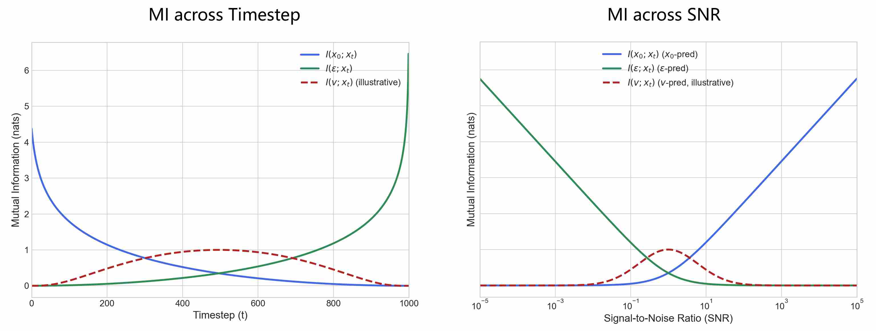
These two charts illustrate the same core issue from two different dimensions: how the information content of different prediction targets is distributed.
Training with $x_0$-prediction is naturally biased toward high-SNR regions, where the model receives the richest signal about the target.
Training with $\epsilon$ or $\text{score}$-prediction is biased toward low-SNR regions, where the input carries the most information about noise.
$v$-prediction avoids over-concentration on either end of the SNR spectrum and instead achieves a more balanced coverage across timesteps. This explains why it often leads to more stable training and perceptually better results in practice.
4. The root causes of instability and inefficiency in diffusion model training
Our information-theoretic analysis revealed how different training targets bias the learning process toward specific regions of the SNR spectrum, and how their mutual information curves explain the uneven distribution of training difficulty. Yet these are only surface manifestations. At a deeper level, the root causes of instability and inefficiency stem from the multi-scale nature of the task: a single neural network is forced to handle objectives that span several orders of magnitude, from high-SNR to low-SNR regimes. This mismatch inevitably leads to imbalanced gradients, irregular optimization dynamics, and uneven learning efficiency.
4.1 The universal perspective of instability and inefficiency
The central challenge of training diffusion models is not a single problem, but a multi-scale one. A single neural network is asked to address a multi-scale problem spanning multiple orders of magnitude. Before introducing concrete stabilization strategies, it is therefore essential to systematically examine these root causes. To do so, we consider two complementary perspectives: the discrete t/SNR-space and the continuous σ-space. Each offers a different lens on where instabilities arise, and clarifies why distinct solution paths—such as re-weighting, scheduling, or preconditioning—are effective.
4.2 From t/SNR-space perspective
When the process is parameterized by discrete timesteps $t$ (or equivalently by SNR), the aboved problem can be reformulated as: different timesteps correspond to highly imbalanced contributions, because the SNR curve induced by the schedule is extremely uneven.
From this perspective, the solution is therefore focus on re-balancing the contribution of timesteps, The goal is to externally adjust the training process to ensure a more uniform and effective contribution from all parts of the denoising chain, we will discuss in section 4.2.
4.3 From σ-space perspective
When the process is parameterized by continuous noise scale $\sigma$, as in EDM 2, the aboved problem can be reformulated as: the target itself changes scale drastically with different noise level, leading to poorly conditioned inputs and outputs unless explicitly normalized.
From this perspective, The solution is therefore focus on reparameterizing and normalizing the task across noise levels, the goal is to re-design the model framework itself to be inherently stable and scale-aware from the ground up, we will discuss in section 4.3.
4.4 Why Different Spaces matters
Distinguishing these two space is critical. It is more than a matter of simple categorization; it reveals the evolution in our understanding of the problem itself. By separating our discussion along these lines, we can clearly understand the motivation, strengths, and limitations of each technique, moving from treating the symptoms to re-engineering the system from first principles.
Although both views tackle the same root cause, they reinterpret the instability differently:
t/SNR-space: imbalance arises from which timesteps are emphasized.
$\sigma$-space: imbalance arises from how the denoiser is conditioned across noise levels.
Because the optimization levers are fundamentally different — scheduling and weighting vs. preconditioning and reparameterization — we will discuss them in separate subsections.
Part III — Stabilizing Diffusion Training
Part II diagnosed diffusion training pathologies as a multi-scale optimization problem: learnable signal and gradient magnitudes are inherently uneven across noise levels, and the same issue appears differently depending on whether we view the process in discrete $t/$SNR space or continuous $\sigma$ space. Part III turns this diagnosis into a set of actionable design principles. Sections 5–9 organize modern stabilization methods into a unified framework: we first introduce a small set of optimization “knobs” that capture most successful interventions (Section 5), then unpack them in depth—how to allocate compute via sampling and schedules (Section 6), how to balance learning via loss weighting (Section 7), how to improve numerical conditioning via preconditioning / parameterization in $\sigma$-space (Section 8), and finally why the architecture itself acts as the vessel that amplifies or bottlenecks all of the above (Section 9).
5. A Unified Framework for Diffusion Model Optimization
As discussed in section 4, the training of diffusion models is inherently a multi-scale optimization problem. Unlike standard supervised learning, where the data distribution is static, diffusion models must learn to reverse a degradation process across a continuum of noise levels—from pristine signals to pure Gaussian noise. This complexity introduces significant instabilities, including gradient imbalance, numerical divergence, and inefficient allocation of computational resources.
Virtually all modern advancements in diffusion stability and efficiency can be distilled into four fundamental axes of optimization.
5.1 Knob 1 — Sampling Optimization: Where to learn
From a stability-and-efficiency perspective, not all noise levels are equally worth spending compute on. A good sampling strategy aims to allocate training steps toward the “useful” region and away from regimes that are effectively wasteful (such as too easy or too hard regimes):
Hence, Knob 1 answers a simple question: Where should we spend our finite training budget across noise levels so that gradients are informative and optimization remains stable?
In many baseline implementations, one samples
\[t \sim \mathrm{Uniform}(0,1),\]constructs $x_t$, and applies the loss at that $t$, this choice is convenient. However, this is suboptimal because the information density of the denoising task is not uniformly distributed.
5.2 Knob 2 — Sampling Optimization: Where to learn
Even with a fixed sampling distribution $p(t)$, gradients can be dominated by certain noise regions because:
- target magnitude varies strongly with noise level;
- the regression difficulty changes with noise level;
- Jacobians / scaling factors (from parameterization) amplify gradients in some regions.
A generic reweighting strategy introduces \(w(t)\) to shape the effective contribution:
\[\mathbb E_{t\sim p(t)}\big[w(t)\,\ell_t(\theta)\big], \qquad \ell_t(\theta) := \mathbb E_{x_0,\epsilon}\big[\ell(\cdot)\big].\]You can interpret $w(t)$ as “how much we care about being correct at this noise level,” but in practice it is more about conditioning the optimization: suppressing gradient explosions, preventing domination by easy/hard regions, and encouraging uniform learning progress.
A crucial theoretical identity is importance sampling:
\[\mathbb E_{t\sim p(t)}[\ell(t)] = \mathbb E_{t\sim q(t)}\left[\frac{p(t)}{q(t)}\,\ell(t)\right].\]This implies that changing sampling \(p(t)\) can be offset by changing weights \(w(t)\) Conversely, a weight function $w(t)$ can be “absorbed” into a new sampling distribution proportional to \(p(t)w(t)\). So “Where to learn” and “How much to learn” are two sides of the same expectation.
5.3 Knob 3 — Conditioning and parameterization: How easy it is to learn
This knob collects techniques that modify the numerical geometry of the regression problem so that learning is stable across noise levels.
Preconditioning: scale the inputs/outputs to reduce ill-conditioning
A core issue is that $x_t$ and the natural targets can have noise-dependent magnitude. If the model sees wildly different scales across $\sigma$, the function it must learn is poorly conditioned; gradients either vanish or explode in some regimes.
Preconditioning addresses this by applying noise-dependent (or noise-aware) scaling to ensure that no matter the noise level $\sigma$, the features entering the residual blocks remain normalized ( zero mean and unit variance, $\mathcal N(0,I)$).
Target parameterization: Instead of predicting the noise $\epsilon$ or the clean image $x_0$ directly—both of which can lead to numerical instability at the boundaries—models are often trained to predict a velocity vector $v$ or a scaled combination. This ensures the output of the network remains within a predictable numerical range, preventing activation saturation and vanishing gradients.
Representation choice: data space vs latent space. Another conditioning lever is the representation in which denoising is learned.
In raw pixel space, the data distribution can be high-dimensional and heavy-tailed; small perturbations can correspond to perceptually large changes.
In a compressed latent space (learned or engineered), the distribution is often smoother and lower-dimensional, and signal energy is more uniformly distributed.
This typically improves stability by reducing the dynamic range of values and gradients; smoothing high-frequency components that are hard to model; making the denoising function “simpler” for the network class.
5.4 Knob 4 — Architectural Scalability: The "Vessel" of Learning
The final axis of optimization concerns the structural integrity of the model itself as it scales to higher resolutions and larger datasets.
As diffusion models transition from U-Nets to Transformers (DiT), new stability challenges arise regarding how information flows through the layers.
Attention Normalization: In high-resolution synthesis, the self-attention mechanism can become a source of instability. Techniques like Query-Key Normalization or FlashAttention are employed to prevent “attention spikes” that can lead to NaN (Not-a-Number) errors during FP16 training.
Positional Robustness: Utilizing Rotary Positional Embeddings (RoPE) or adaptive normalization layers (AdaLN) allows the model to maintain structural coherence across varying aspect ratios and scales, ensuring that the “geometric” part of the denoising process remains stable.
6. Knob 1 — Sampling Optimization: Where to learn
As we discussed in Section 5.1, sampling $t$ uniformly from $[0, T]$ is suboptimal because the information density of the denoising task is not uniformly distributed.
Most of the time, the two endpoints are either extremely simple or extremely difficult. Therefore, the simplest modification is to change the sampling of $t$ from Uniform distribution to Gaussian sampling, and allocate more computational resources to the intermediate time periods. It can also be modified to a more complex sampling method if necessary.
But a more critical issue is that we cannot determine the signal intensity and noise intensity at the current moment solely from the time $t$, nor can we tell whether this moment falls into a high-yield region or a low-yield region. Therefore, in practice, a more useful strategy is to map it to the SNR space or the noise space.
Both SNR and noise can be expressed as functions of $t$. The change-of-variables theorem below indicates that sampling in the t-space, SNR-space, and noise-space is essentially equivalent.
6.1 The Change of Variables Perspective
To make the above precise, introduce a noise-level coordinate $u$. Typical choices include
- $u = \sigma$: (noise standard deviation),
- \(u = \mathrm{SNR} = \alpha(t)^2/\sigma(t)^2\),
- \(u = \lambda = \log\mathrm{SNR}\).
In essentially all diffusion parameterizations used in practice, \(u\) is a deterministic (often monotone) function of \(t\). Write \(u = g(t).\) Now consider an expectation over training time:
\[\mathbb E_{t\sim p_t(t)}[F(g(t))].\]If $g$ is monotone (so it is invertible almost everywhere), we can change variables to $u$. By the change-of-variables theorem, where the induced density over $u$ is
\[p_u(u) \;=\; p_t(t(u))\left|\frac{dt}{du}\right|.\]This identity has two important implications:
Sampling in $t$, $\sigma$, or $\mathrm{SNR}$ is fundamentally equivalent.
Sampling can be done in two interchangeable ways.
Directly choose a desired density $p_u(u)$ in a meaningful noise coordinate \(u\in{\sigma,\mathrm{SNR},\log\mathrm{SNR}}\), then sample $u$ and map back to $t$.
\[\mathbb E_{t\sim p_t(t)}[\mathcal L(t, x_t; \theta)] = \mathbb E_{\sigma\sim p_\sigma}[\mathcal L(\mathrm{SNR}, x_{\mathrm{SNR}}; \theta)] = \mathbb E_{\mathrm{SNR}\sim p_{\mathrm{SNR}}}[\mathcal L(\sigma, x_{\sigma}; \theta)]\]Indirectly keep \(t\sim\mathrm{Uniform}(0,1)\) but redesign the mapping $u=g(t)$ so that the induced \(p_u(u)\propto \|dt/du\|\) matches your desired emphasis.
6.2 Noise schedules is Indirect Sampling
Direct sampling is straightforward, while indirect sampling is more ingenious. Even if $t$ is sampled uniformly, modifying the noise schedule alone can ensure corresponding changes in the noise space. We use the noise schedule in the sigma space as an example to illustrate this point.
Example 1: Linear noise schedule is equal to uniform $\sigma$. Assume we sample time uniformly:
\[t \sim \mathrm{Uniform}(0,1), \qquad \sigma \in [\sigma_{\min},\sigma_{\max}].\]Define a linear noise schedule:
\[\sigma = \sigma_{\min} + t(\sigma_{\max}-\sigma_{\min}).\]Invert it:
\[t(\sigma)=\frac{\sigma-\sigma_{\min}}{\sigma_{\max}-\sigma_{\min}} \qquad \Longrightarrow \qquad \frac{dt}{d\sigma}=\frac{1}{\sigma_{\max}-\sigma_{\min}}.\]By the change-of-variables formula:
\[p_\sigma(\sigma)=p_t(t(\sigma))\left|\frac{dt}{d\sigma}\right|=\underbrace{\frac{1}{\sigma_{\max}-\sigma_{\min}}}_{\text{const}}.\]with \(\sigma\in[\sigma_{\min},\sigma_{\max}].\) So uniform sampling in (t) induces uniform sampling in (\sigma) under a linear schedule.
Example 2: Log-linear (exponential) schedule is equal to log-uniform $\sigma$. Again we let \(t \sim \mathrm{Uniform}(0,1).\) Define a log-linear schedule (i.e., \(\log \sigma\) is linear in \(t\)):
\[\sigma = \sigma_{\min}\left(\frac{\sigma_{\max}}{\sigma_{\min}}\right)^t.\]Invert it:
\[t(\sigma)=\frac{\ln(\sigma/\sigma_{\min})}{\ln(\sigma_{\max}/\sigma_{\min})} \quad \Longrightarrow \quad \frac{dt}{d\sigma} = \frac{1}{\sigma\,\ln(\sigma_{\max}/\sigma_{\min})}.\]Apply change-of-variables:
\[p_\sigma(\sigma)=p_t(t(\sigma))\left|\frac{dt}{d\sigma}\right| = \frac{1}{\sigma\,\ln(\sigma_{\max}/\sigma_{\min})}, \qquad \sigma\in[\sigma_{\min},\sigma_{\max}].\]This density satisfies \(p_\sigma(\sigma)\propto 1/\sigma\), which is exactly log-uniform: if we define \(u=\ln\sigma\), then
\[u \sim \mathrm{Uniform}(\ln\sigma_{\min}, \ln\sigma_{\max}).\]The two examples mentioned above demonstrate that even if $t$ is sampled uniformly, modifying the noise schedule can indirectly alter the sampling in the $\sigma$-space, thereby achieving the effect of stability training.
6.3 Noise schedules
In t-space parameterization, stability is tightly linked to how the noise schedule is designed. The forward process is defined through a sequence of variance increments ${\beta_t}_{t=1}^T$, which accumulate into $\alpha_t$ and $\bar\alpha_t$. Different choices of $\beta_t$ correspond to different trajectories of signal-to-noise ratio (SNR) as training progresses.
Linear schedule: This is the original implementation of DDPM 3, $\beta_t$ increases linearly from a small value $\beta_{min}$(e.g. $10^{-4}$) to a larger value $\beta_{max}$ (e.g. $0.02$).
\[\beta_t = \beta_{\text{min}} + (t - 1) \cdot \frac{\beta_{\text{max}} - \beta_{\text{min}}}{T - 1}, \quad t = 1, 2, \dots, T\]Scaled Linear Schedule: A variant of the linear schedule, tailored for latent diffusion models (e.g., Stable Diffusion). It scales the betas by taking the square root of the range, linearly interpolating, and then squaring the result. This creates a non-linear growth curve where betas start smaller and increase more gradually initially, helping with stability in latent spaces where noise scales differently. It’s particularly useful for models trained on compressed representations to avoid over-noising early timesteps.
\[\beta_t = \left( \sqrt{\beta_{\text{min}}} + (t - 1) \cdot \frac{\sqrt{\beta_{\text{max}}} - \sqrt{\beta_{\text{min}}}}{T - 1} \right)^2, \quad t = 1, 2, \dots, T\]In latent diffusion models (LDMs), the scaled linear noise schedule is preferred over the original linear schedule for several important reasons:
In latent space, because the representation has lower variance, using the same $\beta$ range (e.g., 0.0001 $\to$ 0.02 in linear schedule) breaks the SNR dynamics, noise is injected too aggressively, and the signal disappears too early, that means the model sees nearly pure noise for a large fraction of training, which is inefficient.
Scaled linear slows down noise growth with a narrower range of $\beta$ values (e.g., 0.00085 $\to$ 0.012 in SD), so that the SNR curve decays more smoothly, balances the learning signal, stabilizes training, and yields higher-quality outputs.
Squaredcos Cap V2 Schedule (Cosine Schedule): This strategy uses a cosine-based function to create a smoother, more gradual increase in noise. Rather than direct definition $\beta$, this relies on an intermediate function for the cumulative alpha $\bar{\alpha}_t$ 4.
\[\bar{\alpha}(t) = \cos^2 \left( \frac{t / T + s}{1 + s} \cdot \frac{\pi}{2} \right), \quad s = 0.008\]And then,
\[\beta_t = \min \left( 1 - \frac{\bar{\alpha}(t)}{\bar{\alpha}(t-1)}, \ \beta_{\max} \right), \quad \beta_{\max} = 0.999\]Exponential Schedule: As the name suggests, the exponential noise schedule defines the rate of noise change in a manner that follows an exponential growth pattern. This schedule is designed to ensure that $\beta$ increases exponentially as the timestep t progresses. The function governing the exponential noise schedule is given by:
\[\beta_t = \beta_{\text{start}} \cdot \left( \frac{\beta_{\text{end}}}{\beta_{\text{start}}} \right)^{\frac{t-1}{T-1}}, \quad t = 1, 2, \dots, T\]Sigmoid Schedule: This strategy uses a sigmoid function to create an S-shaped curve for $\beta_t$, starting near $\beta_{\text{min}}$, rising steeply in the middle, and plateauing near $\beta_{\text{max}}$. It’s particularly useful for tasks requiring rapid noise increase in mid-timesteps (e.g., GeoDiff or inpainting models), offering better control over multi-scale noise addition and improving training stability.
\[\beta_t = \sigma \left( -6 + 12 \cdot \frac{t-1}{T-1} \right) \cdot (\beta_{\text{end}} - \beta_{\text{start}}) + \beta_{\text{start}}, \quad t = 1, 2, \dots, T\]where $\sigma(x) = \frac{1}{1 + e^{-x}}$ is the logistic sigmoid function, scaled from -6 to 6 to cover the full range.
We plot a direct comparison of the SNR curves for these noise schedulers.
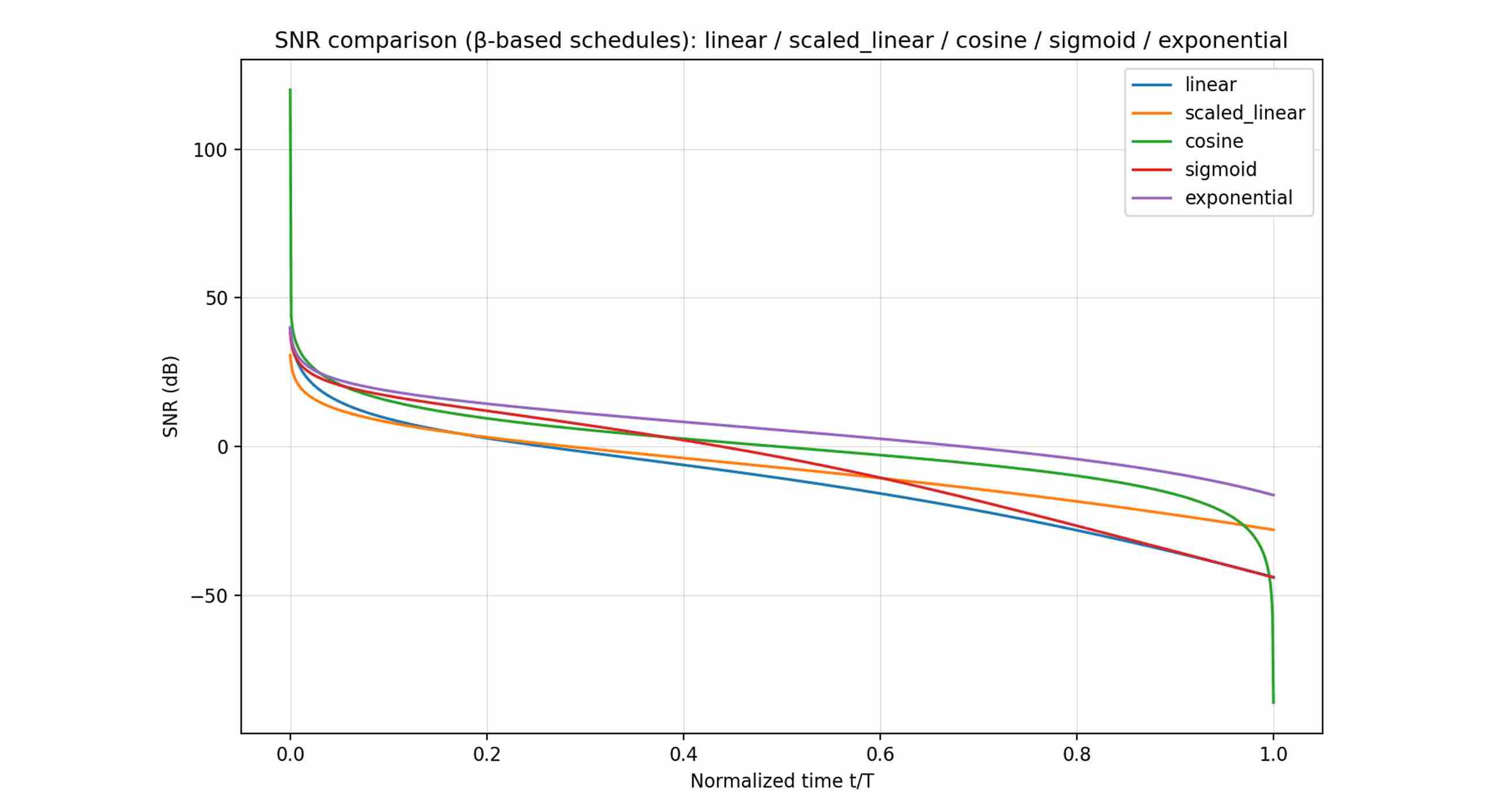
Many common β-schedules (linear, cosine, etc.) leave a small non-zero SNR at the last step. During training the model learns to exploit this residual signal, but during inference we usually start from pure noise. This mismatch causes artifacts like limited brightness or reduced dynamic range.
Zero Terminal SNR (ZTSNR) 5 is an effective solution to this problem, which enforces the SNR at the final timestep $\text{SNR}(T)=0$ to be exactly zero — i.e., the sample at the terminal step should be pure Gaussian noise without any residual data signal.
Implementing ZTSNR in diffusion models involves modifying the noise schedule to ensure that the cumulative product of alphas ($\bar{\alpha}_T$) reaches zero at the terminal timestep $T$, effectively setting the SNR to zero.
\[\bar{\alpha}_T=0\,\qquad\,\text{SNR}(T)=\frac{\bar{\alpha}_T}{1- \bar{\alpha}_T}=0\]One effective method is to rescale the $\beta_t$ values to adjust the cumulative alpha product.
\[\beta_t' = \beta_t \cdot \frac{1 - \bar{\alpha}_1}{1 - \bar{\alpha}_T}\]Recalculate $\alpha_t’ = 1 - \beta_t’$ and \(\bar{\alpha}_t' = \prod_{i=1}^t \alpha_i'\), verifying that \(\bar{\alpha}_T' \approx 0\). This scales the original betas to ensure $\bar{\alpha}_T$ approaches zero while preserving the relative shape of the schedule.
7. Knob 2 — Loss Weighting: How much to learn
The most direct way to counteract imbalanced learning is to apply a weighting term $w(t)$ to the loss function, making the objective:
\[\mathcal{L}_{w} = \mathbb{E}_{t, x_t} \left[ w(t)\|y_t - f_{\theta}(x_t, t)\|^2 \right]\label{eq:39}\]Where $w(t)=1$ in our previous discussion (vanilla diffusion training). The function $w(t)$ acts as a precision-engineered “equalizer” for our training process. It amplifies the learning signal where it’s naturally weak and suppress the loss when the gradient variance is large to prevent instability. The goal is to design $w(t)$ such that the effective learning task is normalized across all timesteps (or all SNR regions), we summarizes several mainstream weighting strategies as follows:
7.1 Perception Prioritized (P2) Weighting
This innovative approach, introduced by Choi et al. 6, shifts the optimization goal from minimizing raw MSE to minimizing human-perceived error, often measured by metrics like LPIPS, where
\[w(t) = \frac{1}{(\kappa + \text{SNR}(t))^\gamma}\]The paper recommends hyperparameters $\kappa=1$ and $\gamma=0.5$. This strategy is born from the observation that MSE is a poor proxy for perceptual quality. The authors found that most of the perceptual error occurs in the mid-to-high SNR range, even when the MSE is low. The P2 weighting scheme is therefore counter-intuitively designed to down-weight the high-SNR regime ($w(t) \to 0$ as $\text{SNR}(t) \to \infty$) and up-weight the mid-to-low SNR regime ($w(t) \approx 1$ as $\text{SNR}(t) \to 0$).
The logic is to force the model to first learn the semantically crucial, large-scale structures of the image (governed by mid-to-low SNR steps) correctly. A well-formed global structure provides a better foundation for generating perceptually pleasing details, even if the MSE in the high-SNR details is not minimized as aggressively.
7.2 SNR-Based weighting
This is a simple, elegant, and effective strategy that provides a balanced solution by weighting the loss directly by the SNR: \(w(t) = \text{SNR}(t)\) 7, Or, more generally, it can be formalized
\[w(t) = (\text{SNR}(t))^{\gamma},\quad \gamma > 0\]This approach cleverly addresses both primary difficulties simultaneously:
- At High SNR: The weight is large, amplifying the weak signal of $\epsilon$-prediction and forcing the model to learn details.
- At Low SNR: The weight is small, suppressing the large and noisy gradients common to $x_0$-prediction, thus promoting stability.
It provides a balanced trade-off, ensuring that neither end of the SNR spectrum dominates the training process. However, due to the potentially large variation range of SNR, using logarithmic scaling ($w(t)=\log(\text{SNR}(t))$) can make the weight distribution across different SNR regions more balanced.
7.3 Min-SNR Weighting
Min-SNR Weighting 8 sets an upper bound to suppress the high-SNR region.
\[w(t) = \min(\text{SNR}(t), \tau)\]In both the official implementation and the Diffusers library, $\tau$ is set to 5 by default.
When $\text{SNR}(t) < \tau$ (Low-to-Mid {SNR} regime): The weight is $w(t) = \text{SNR}(t)$. The behavior is identical to standard SNR weighting.
When $\text{SNR}(t) \geq \tau$ (High SNR regime): The weight is “capped” at a constant upper bound, $w(t) = \tau$. It no longer increases as the SNR grows.
A massive weight in high-SNR area can cause the model to focus excessively on minuscule errors in high-frequency details. This can result in perceptually unpleasant artifacts, such as “over-sharpened” or “fried” textures, which harm the naturalness of the generated image. Min-SNR strategy acts as a “limiter” on the signal amplifier. It ensures that the model learns details sufficiently without the detrimental side effects of extreme weights.
This balancing prioritizes better perceptual quality and training stability by preventing the model from becoming pathologically focused on details.
7.4 Max-SNR Weighting
Max-SNR Weighting 9 sets an lower bound to ensure a minimum learning signal.
\[w(t) = \max(\text{SNR}(t), \tau)\]When $\text{SNR}(t) > \tau$ (Mid-to-High SNR regime): The weight is $w(t) = \text{SNR}(t)$. In this range, the behavior is identical to standard SNR weighting, leveraging a high weight to amplify the weak signal in the high-SNR region.
When $\text{SNR}(t) \leq \tau$ (Very Low SNR regime): The weight is “frozen” at a constant lower bound, $w(t) = \tau$. It no longer approaches zero as the SNR decreases.
When the weight is approach to 0 (in low-snr area), the model might learn that it receives no penalty for errors in these initial steps and therefore fails to learn how to meaningfully begin the denoising process. This can hinder the start of the generation or lead to artifacts in the final sample. Max-SNR strategy enforces a minimum level of supervision even in the noisiest regimes, and compels the model to learn a meaningful “first step” out of the noise distribution.
Overall, This balancing prevents a “blind spot” in the learning process, ensuring the integrity and effectiveness of the entire denoising chain from pure noise to clean image.
7.5 SNR clipping
This strategy is a robust combination of the previous two.
\[w(t) = \min(\max(\text{SNR}(t), \tau_{min}), \tau_{max})\]- When $\text{SNR}(t) < \tau_{min}$ (Very Low SNR): $w(t) = \tau_{min}$ (the floor is active).
- When $\tau_{min} \leq \text{SNR}(t) \leq \tau_{max}$ (Core SNR range): $w(t) = \text{SNR}(t)$ (standard behavior).
- When $\text{SNR}(t) > \tau_{max}$ (Very High SNR): $w(t) = \tau_{max}$ (the ceiling is active).
This strategy boosts the weights in the lowest SNR region and suppresses them in the highest SNR region, effectively creating a trapezoidal weighting curve. Theoretically speaking, it simultaneously optimize the learning signal, gradient stability, and perceptual quality. It is one of the most robust heuristic weighting schemes in practice.
8. Knob 3 — Conditioning and parameterization: How easy it is to learn
In this section, we discuss the $\sigma$-space approach who treats instability as a conditioning and reparameterization problem.
8.1 EDM-Style Preconditioning
In early diffusion models such as DDPM or DDIM, both training and sampling were defined in terms of a discrete timestep $t \in {1,\dots,T}$. A noise schedule ${\beta_t}$ was chosen, then transformed into $\alpha_t$ and $\bar{\alpha}_t$, and the network was trained with $t$ as its input.
The limitation of this viewpoint is that the relationship between SNR and timestep $t$ depends entirely on the chosen schedule (linear, cosine, exponential, etc.). As a result, the effective learning task is schedule-dependent: the same $t$ can correspond to vastly different SNR levels and hence very different learning difficulties.
8.1.1 From $t$-space to $\sigma$-space
EDM introduces a critical shift: instead of modeling in the discrete timestep space, all training objectives and parameterizations are expressed directly in terms of the continuous noise scale $\sigma$. Consequently, a noisy data point at any noise level is elegantly expressed as:
\[x(\sigma) = x_0 + \sigma \,\epsilon, \quad \epsilon \sim \mathcal N(0,I).\]Here $\sigma$ is the standard deviation of the added Gaussian noise. It is directly linked to the signal-to-noise ratio (SNR):
\[\text{SNR} = \frac{1}{\sigma^2}.\]Important: All subsequent design choices—preconditioning coefficients, loss weights, training distributions—are defined as functions of $\sigma$ rather than $t$.
8.1.2 Preconditioning Formulation
The previous section on Strategic Loss Weighting aimed to correct the training objective, balancing the model’s focus across different SNR regimes. However, the root of instability lies not just in the objective function but is also deeply embedded in how the network architecture handles inputs and outputs of dramatically varying scales.
From our “$\sigma$-space perspective”, the instability of network training becomes exceptionally clear: as $\sigma$ varies from very small to very large values, the variance of the network input $x_t$, given by ${\text Var}(x_t) = {\text Var}(x_0) + \sigma_t^2$, and the scales of various potential prediction targets (like $x_0$ or $\epsilon$) change dramatically, often across several orders of magnitude.
Demanding a single, fixed neural network $f_θ$ to effectively process inputs with a magnitude of $0.1$ in one forward pass and $100$ in another—while its output target undergoes similar wild fluctuations—poses a tremendous challenge for the optimizer and the network weights. This can lead to exploding or vanishing gradients at different timesteps, severely undermining training stability.
To remove scale inconsistencies across different noise levels, Karras et al. 2 introduced a pivotal technique: Network Pre-conditioning. The core idea is to use simple, analytically-defined scaling functions to “normalize” the network’s inputs and outputs. This ensures the core network $f_{\theta}$ always operates in a well-behaved “comfort zone” where its inputs and outputs have roughly constant, near-unit variance.. EDM expresses the pre-conditioned network (also known as denoiser, the target is $x_0$) as:
\[F_{\theta}(x(\sigma), \sigma) = c_{\text{out}}(\sigma)\, f_{\theta}(c_{\text{in}}(\sigma) \, x(\sigma), \, c_{\text{noise}}(\sigma)) + c_{\text{skip}}(\sigma) \, x(\sigma)\]Here, $f_θ$ is our core U-Net architecture, and the $c_…$ terms are simple scalar functions that depend only on the noise level $\sigma$. Let’s precisely break down this formula in $\sigma$-space:
$c_{\text{in}}(\sigma)$ (Input Scaling): This term aims to counteract the scale variation of the input $x(σ)$. To give $f_{\theta}$’s input a constant variance, $c_{\text{in}}(\sigma)$ must cancel out the variance of $x(\sigma)$. Letting the clean data variance be $\sigma_{\text {data}}^2 = \mathrm{Var}(x_0)$, we have $\mathrm{Var}(x(\sigma)) = \sigma_{\text {data}}^2 + \sigma^2$. EDM therefore chooses:
\[c_{\text{in}}(\sigma) = \frac{1}{\sqrt{\sigma^2 + \sigma_{\text data}^2}}\]which ensures that the U-Net sees inputs with similar statistical properties regardless of $\sigma$.
$c_{\text{noise}}(\sigma)$ (Noise Level Encoding): The continuous value of $\sigma$ (typically a transformation of its logarithm, like
\[c_{\text{noise}}(\sigma) = 0.25 \log(\sigma)\]which is fed directly as the conditioning, replacing discrete $t$ embeddings. This allows the network to reason over a continuum of noise levels.
The noise conditioning variable $c_{\text{noise}}$ in EDM is defined as a logarithmic function of the noise level, typically $c_{\text{noise}} = 0.25 \log \sigma $, to achieve numerical stability and smooth conditioning across a wide dynamic range of noise scales. Since $\sigma$ in diffusion models can vary over several orders of magnitude (e.g., from $10^{-3}$ to $10^{3}$), using the raw value would make the model highly sensitive and difficult to train. Representing the noise level in log-space compresses this range into a roughly linear and well-behaved domain, allowing the network to learn a smoother and more uniform mapping between noise intensity and denoising behavior. In addition, the scaling factor $0.25$ (not strict) keeps the magnitude of $c_{\text{noise}}$ within a range suitable for neural modulation layers, ensuring stable gradients and consistent conditioning across all noise levels.
$c_{\text{skip}}(\sigma)$ (Skip Scaling): This is the most ingenious part of the pre-conditioning framework. Let’s consider the expression of pre-conditioned network $F_{\theta}$. We notice that it consists of two components: one is the linear part, and the other is the nonlinear part. This semi-linear structure is crucial in the training and sampling of diffusion models.
\[F_{\theta}(x(\sigma), \sigma) = \underbrace{c_{\text{skip}}(\sigma) \cdot x(\sigma)}_{\text{Linear Baseline Prediction}} + \underbrace{c_{\text{out}}(\sigma) \cdot f_{\theta}(c_{\text{in}}(\sigma) \cdot x(\sigma), c_{\text{noise}}(\sigma))}_{\text{Non-linear Residual Correction}}\]Now, the meaning of $c_{\text{skip}}(\sigma) \cdot x(\sigma)$ is very clear: $c_{\text{skip}}(\sigma) \cdot x(\sigma)$ is the best linear estimate of the target signal ($x_0$) given the noisy input $x(\sigma)$. And as we learned in Section 3.2, in the sense of minimizing the mean squared error, this best linear estimate is the conditional expectation $\mathbb{E}[x_0 \mid x(\sigma)]$. The solution for $\mathbb{E}[x_0 \mid x(\sigma)]$ can be obtained through Equation.
\[\begin{align} \mathbb{E}(x_0 \mid x(\sigma)) & = \mathbb{E}(x_0) + \frac{\mathrm{Cov}(x_0, x(\sigma))}{\mathrm{Var}(x(\sigma))}\left( x(\sigma) - \mathbb{E}(x(\sigma)) \right) \\[10pt] & = 0 + \frac{\mathrm{Cov}(x_0, x_0+\sigma\,\epsilon)}{\mathrm{Var}(x(\sigma))}\left( x(\sigma) - 0 \right) \\[10pt] & = \frac{\sigma_{\text data}^2}{\sigma_{\text data}^2 + \sigma^2}\,x(\sigma) \end{align}\]this implies the best choice of $c_{\text{skip}}(\sigma)$.
\[c_{\text{skip}}(\sigma) = \frac{\sigma_{\text data}^2}{\sigma_{\text data}^2 + \sigma^2}\]$c_{\text{out}}(\sigma)$ (output Scaling): Since $c_{\text{skip}}$ has handled the linear part, what is left for the expensive U-Net $f_{\theta}$ to learn? It must learn the difference: the non-linear residual. By rearranging the pre-conditioning formula, we can see the learning target for $f_{\theta}$:
\[f_{\theta} \approx \frac{x_0 - c_{\text{skip}}(\sigma) \cdot x(\sigma)}{c_{\text{out}}(\sigma)}\]The numerator, $x_0 - c_{\text{skip}}(\sigma)\,x(\sigma)$, represents the error between the true signal $x_0$ and its best linear estimate. However, the variance of this error still changes dramatically with $\sigma$. If $f_{\theta}$ were to learn this error directly, its output scale would remain unstable. Specifically, we want the variance of $f_{\theta}$ is 1, this implies the choice of $c_{\text{out}}(\sigma)$ is.
\[\begin{align} c_{\text{out}}(\sigma) & = \sqrt{ \mathrm{Var}(x_0) + c_{\text{skip}}^2(\sigma)\mathrm{Var}(x(\sigma)) - 2{\mathrm Cov(x_0, c_{\text{skip}}x_{\sigma})} }\\[10pt] & = \sqrt{\sigma_{\text{data}}^2+c_{\text{skip}}^2(\sigma_{\text{data}}^2+\sigma^2)-2c_{\text{skip}}\sigma_{\text{data}}^2} \\[10pt] & = \frac{\sigma\,\sigma_{\text {data}}}{\sqrt{\sigma_{\text {data}}^2 + \sigma^2}} \end{align}\]
8.1.3 EDM as a Unified Interface for different targets
An important perspective is that the preconditioned network $F_\theta$ acts as a unified interface (or container). Regardless of which prediction target we prefer — $x_0$, $\epsilon$, $v$, or the score — all can be obtained from $F_\theta$ by a fixed linear transformation.
| Prediction target | Expression in terms of $F_\theta(x;\sigma)$ | Notes |
|---|---|---|
| Clean data ($x_0$) | $\hat x_0 = F_\theta(x;\sigma)$ | $F_\theta$ is default designed as an denoiser, i.e. the optimal estimate of $x_0$. |
| Noise ($\epsilon$) | $\hat\epsilon = \frac{x - F_\theta(x;\sigma)}{\sigma}$ | Direct inversion of the corruption process $x = x_0 + \sigma\epsilon$. |
| Score ($\nabla_x \log p(x;\sigma)$) | $s(x;\sigma) = \frac{F_\theta(x;\sigma) - x}{\sigma^2}$ | EDM’s denoising–score matching identity. |
| $v$-prediction | $\hat v = \hat\epsilon - \sigma\,\hat x_0$ | $v$ is a linear combination of $(x_0,\epsilon)$; coefficients $a(\sigma), b(\sigma)$ depend on the forward process. |
Meanwhile, $f_\theta$ itself is not any of these targets. It is purely a residual learner operating under normalized conditions. No matter which target we adopt, $f_\theta$ always sees input and supervision with variance $\approx$ 1, and learns a goal-agnostic residual. This design delivers stability in multiple ways:
- Normalized inputs ($c_{\text{in}}$): consistent scale for all $\sigma$.
- Uniform outputs ($c_{\text{out}}$): targets with equalized variance.
- Balanced skip path ($c_{\text{skip}}$): statistically optimal linear baseline, reducing residual magnitude.
- Stable noise embedding ($c_{\text{noise}}$): well-scaled conditioning variable.
- Target-agnostic residual learning: by treating $D_\theta$ as a universal interface, EDM guarantees that switching objectives does not destabilize $F_\theta$’s training.
Preconditioning Coefficients for Different Targets
| Prediction target | $c_{\text{skip}}(\sigma)$ | $c_{\text{out}}(\sigma)$ | $c_{\text{in}}(\sigma)$ | $c_{\text{noise}}(\sigma)$ |
|---|---|---|---|---|
| $x_0$ | $\dfrac{\sigma_{\text{data}}^2}{\sigma_{\text{data}}^2+\sigma^2}$ | $\dfrac{\sigma\,\sigma_{\text{data}}}{\sqrt{\sigma_{\text{data}}^2+\sigma^2}}$ | $\dfrac{1}{\sqrt{\sigma_{\text{data}}^2+\sigma^2}}$ | $\tfrac14\ln\sigma$ |
| $\epsilon$ | $\dfrac{\sigma}{\sigma_{\text{data}}^2+\sigma^2}$ | $\dfrac{\sigma_{\text{data}}}{\sqrt{\sigma_{\text{data}}^2+\sigma^2}}$ | $\dfrac{1}{\sqrt{\sigma_{\text{data}}^2+\sigma^2}}$ | $\tfrac14\ln\sigma$ |
| $v$ | $0$ | $1$ | $\dfrac{1}{\sqrt{\sigma_{\text{data}}^2+\sigma^2}}$ | $\tfrac14\ln\sigma$ |
| score | $-\dfrac{1}{\sigma_{\text{data}}^2+\sigma^2}$ | $\dfrac{\sigma_{\text{data}}}{\sigma\sqrt{\sigma_{\text{data}}^2+\sigma^2}}$ | $\dfrac{1}{\sqrt{\sigma_{\text{data}}^2+\sigma^2}}$ | $\tfrac14\ln\sigma$ |
8.2 Sigma sampling distributions
Along the new preconditioning network $F_{\theta}$, and given a chosen training target $T(\sigma)$ (which may be $x_0,\ \epsilon,\ v,$ or the score), we reconstruct the loss function.
\[\boxed{\quad \mathcal{L}(\theta) =\mathbb{E}_{\sigma\sim p(\sigma)}\ \mathbb{E}_{x_0,\epsilon}\left[ \lambda(\sigma)\ \big\|\,F_\theta(x;\sigma)-T(\sigma)\,\big\|_2^2 \right].\quad}\]where $p(\sigma)$ is the sigma sampling distribution, and $\lambda(\sigma)$ is the loss weight. The primary difference from Equation \ref{eq:39} lies in the fact that we sample in the $\sigma$ space rather than the t space.
Once the EDM-style preconditioning framework is in place, the next critical design choice concerns how to sample the noise scale $\sigma$ during training. Unlike classical diffusion models, which typically draw timesteps $t$ uniformly from $[0,1]$, EDM samples $\sigma$ values directly from a log-normal distribution. This subtle change dramatically improves training stability and efficiency.
In the following discussion, we examine three sampling strategies: Linear Uniform, $\log$ Uniform, and $\log$ Normal. All sampling strategies are performed within the interval from $\sigma_{\text min}=0.002$ to $\sigma_{\text max}=80$.
8.2.1 The Naive Approach: Linear Uniform Sampling on $\sigma$
The simplest and most intuitive way to train a model across a range of noise levels from $\sigma_{\text min}$ to is to sample $\sigma$ uniformly from this interval. While mathematically simple, this approach is disastrously inefficient from an information-theoretic perspective. The core problem is that linear distance in $\sigma$-space does not correspond to a linear change in learning difficulty or perceptual quality. Let’s consider the range $[0.002, 80]$.
- The sub-interval $[40, 80]$ has a length of 40.
- The sub-interval $[0.002, 40.002]$ also has a length of 40.
Under a linear uniform sampling scheme, these two intervals will receive an equal number of training samples—approximately 50% of the total training budget each. However, this two sub-intervals are equal in terms of distance, but unbalanced in terms of information.
- In $\sigma \in [40, 80]$: The noise term $\sigma \epsilon$ completely dominates the data term $x_0$. The SNR is exceptionally low. The model is essentially tasked with reconstructing a masterpiece from a blizzard of pure static. It can only learn the coarsest, most averaged-out features of the data distribution. A vast amount of computational resource is spent on a pure noise region with minimal learning value.
- In $\sigma \in [0.002, 40.002]$: This single interval contains the entire meaningful learning journey. It’s where the model learns to form global structures ($\sigma \approx 30$), define semantic content ($\sigma \approx 10$), add textures and medium-frequency details ($\sigma \approx 1$), and perform final, high-fidelity refinement ($\sigma \approx 0.1$).
By sampling $\sigma$ linearly, we force the model to spend half its time learning from static, effectively wasting a massive portion of the training budget.
8.2.2 A Major Leap Forward: Log-Uniform Sampling
The fundamental flaw of the linear approach is its failure to recognize that noise levels are best understood in terms of orders of magnitude. The perceptual difference between $\sigma=0.1$ and $\sigma=1$ is far more significant than the difference between $\sigma=70.1$ and $\sigma=71$. This insight leads us directly to the logarithmic scale.
Instead of sampling $\sigma$ uniformly, we sample $\log(\sigma)$ uniformly from the interval $[\log(\sigma_{\text min}), \log(\sigma_{\text max})]$. This is equivalent to $\sigma$ following a Log-Uniform distribution.
This change in perspective is transformative. Let’s revisit our comparison:
- The interval $[0.1, 1]$ in log-space has a “length” of $\log(1) - \log(0.1) \approx 2.3$.
- The interval $[1, 10]$ in log-space has a “length” of $\log(10) - \log(1) \approx 2.3$.
- The interval $[10, 80]$ in log-space has a “length” of $\log(80) - \log(10) \approx 2.08$.
Under Log-Uniform sampling, these intervals—representing distinct orders of magnitude—receive a roughly equal allocation of training samples. This aligns perfectly with the denoising task. The model now spends a balanced amount of effort learning to:
- Transition from high noise to medium noise (e.g., $\sigma=10 \quad \to \quad \sigma=1$).
- Transition from medium noise to low noise (e.g., $\sigma=1 \quad \to \quad \sigma=0.1$).
On a log-scaled histogram, this distribution appears flat, confirming that each decade of σ is treated with equal importance. This strategy rectifies the catastrophic misallocation of the linear uniform approach and provides a robust, principled, and parameter-free (besides the boundaries) baseline.
8.2.3 The EDM Approach: Log-Normal Sampling
Log-Uniform sampling is a massive improvement, but it rests on a new assumption: that all orders of magnitude are equally important to learn from.
There is likely a “sweet spot”—a critical phase in the denoising process where the most complex and semantically meaningful features of the data are learned. Log-Normal Sampling strategy proposes that $\log(\sigma)$ should not be sampled uniformly, but from a Normal (Gaussian) distribution:
\[\log(\sigma) \sim \mathcal{N}(P_{\text{mean}}, P_{\text{std}}^2)\]Consequently, $\sigma$ itself follows a Log-Normal distribution. This approach abandons the idea of equal effort and instead adopts a strategy of focused learning. The Gaussian distribution in log-space creates a peak, concentrating the majority of training samples around a specific noise level, with density tapering off towards the extremes.
- Targeting the “Sweet Spot”: The key is that the denoising task is not uniformly difficult across scales.
- High-$\sigma$ Regime: Learning coarse, global layouts. The task is relatively simple.
- Mid-$\sigma$ Regime: This is often the most critical phase. The model transitions from abstract blobs to recognizable semantic content—forming faces, defining objects, creating complex textures. This is arguably the most difficult and information-rich part of the process.
- Low-$\sigma$ Regime: Fine-tuning, removing minor artifacts, and adding high-frequency texture. This is a refinement task.
The Log-Normal distribution, by choosing an appropriate $P_{\text {mean}}$ (e.g., -1.2 in the EDM paper, corresponding to $\sigma \approx 0.3$), focuses the model’s training effort squarely on the crucial mid-to-low $\sigma$ regime where core content is synthesized.
- Introducing Control via Hyperparameters: The apparent downside of this approach is the introduction of two hyperparameters, $P_{\text {mean}}$ and $P_{\text {std}}$. However, these are not arbitrary constants but powerful design knobs:
- $P_{\text {mean}}$: This parameter acts like a spotlight, setting the center of gravity for the training process. It allows researchers to target the most relevant noise scale for a given task.
- $P_{\text {std}}$: This parameter controls the focus of the spotlight. A small $P_{\text {std}}$ creates a tight, focused distribution for tasks that operate in a narrow $\sigma$ range (e.g., super-resolution). A larger $P_{\text {std}}$ creates a broader distribution, closer to Log-Uniform, suitable for general-purpose image generation.
We apply these three sampling strategies respectively for sampling. Based on 500,000 samplings, a unified log-space histogram will be obtained
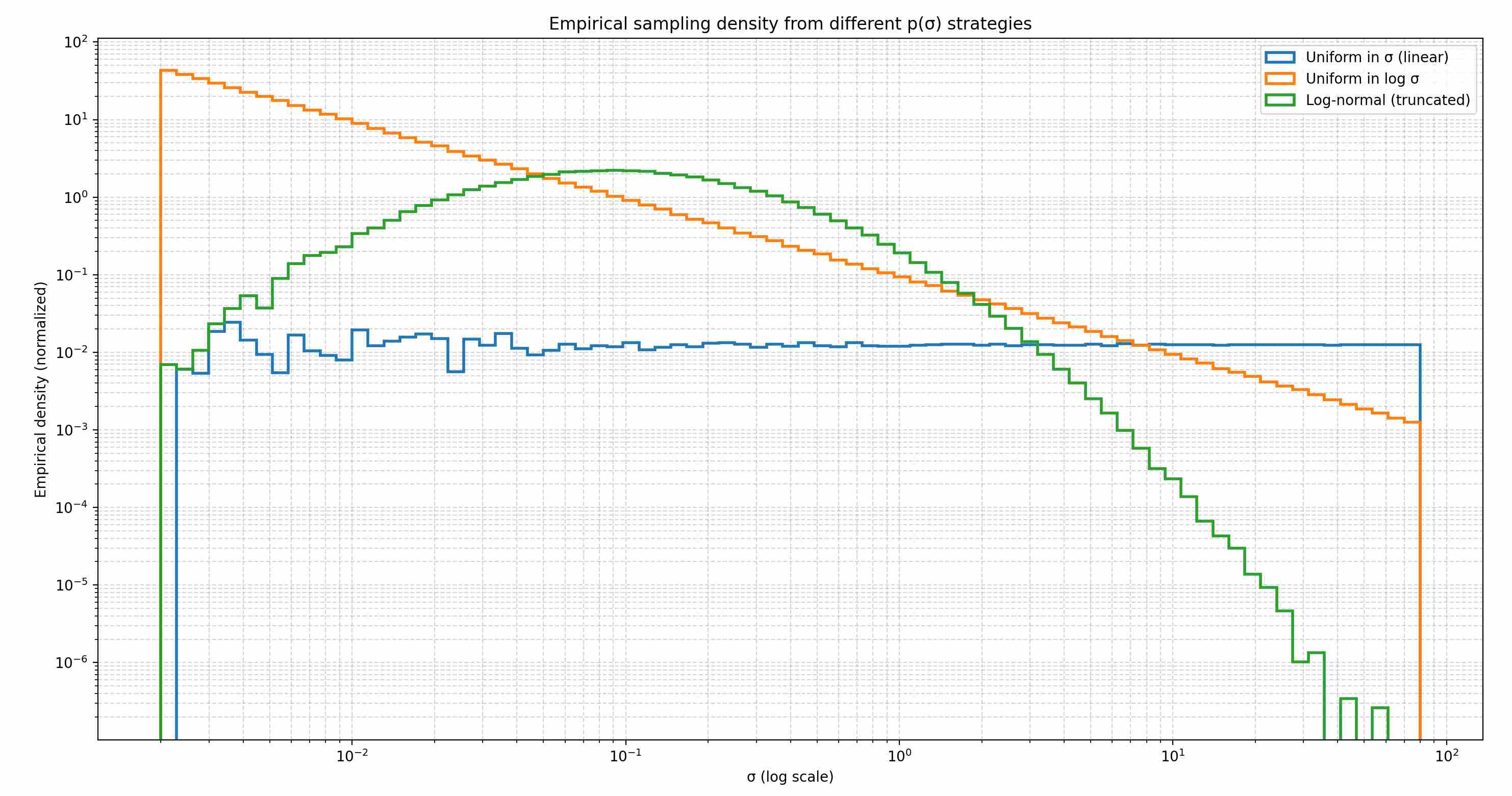
Linear Uniform: although flat in linear space, it allocates the majority of samples to the large-$\sigma$ end, since that region spans most of the interval.
Log Uniform: distributes training budget approximately equally across each order of magnitude, giving all noise scales comparable attention.
Log-normal: concentrates sampling density around the mid-range near $\sigma \approx 0.3$, where residuals are most informative, while still maintaining coverage of both low- and high-noise extremes.
8.3 Loss weighting in $\sigma$-space
Even with a good sampling distribution, contributions across $\sigma$ can still be skewed unless losses are normalized. Returning to the preconditioned head. Define the normalized residual
\[R(\sigma)=\frac{T(\sigma)-c_{\text{skip}}(\sigma)\,x}{c_{\text{out}}(\sigma)}.\]Then the loss can be written as
\[\begin{align} \mathcal{L}(\theta) & =\mathbb{E}_{\sigma\sim p(\sigma)}\ \mathbb{E}_{x_0,\epsilon}\Big[ \lambda(\sigma)\ \big\|\,F_\theta(x;\sigma)-T(\sigma)\,\big\|_2^2 \Big] \\[10pt] & = \mathbb{E}_{\sigma\sim p(\sigma)}\ \mathbb{E}_{x_0,\epsilon}\Big[ \lambda(\sigma)\ \big\|\, c_{\text{out}}f_{\theta}(c_{\text{in}}x, c_{\text{noise}}) + c_{\text{skip}}\,x-T(\sigma)\,\big\|_2^2 \Big] \\[10pt] & = \mathbb{E}_{\sigma\sim p(\sigma)}\ \mathbb{E}_{x_0,\epsilon}\Big[ \lambda(\sigma)\,c_{\text{out}}(\sigma)^2 \big\|f_\theta(c_{\text{in}}x;\ c_{\text{noise}})-{\frac{T(\sigma)-c_{\text{skip}}(\sigma)\,x}{c_{\text{out}}(\sigma)}}\big\|^2 \Big] \\[10pt] & = \mathbb{E}_{\sigma\sim p(\sigma)}\ \mathbb{E}_{x_0,\epsilon}\Big[ \lambda(\sigma)\,c_{\text{out}}(\sigma)^2 \big\|f_\theta(c_{\text{in}}x;\ c_{\text{noise}})-R(\sigma)\big\|^2 \Big] \end{align}\]EDM set
\[\lambda(\sigma)={1}/{c_{\text{out}}(\sigma)^2},\]so that the factor cancels, leaving
\[\mathcal{L}(\theta) =\mathbb{E}_{\sigma\sim p(\sigma)}\ \mathbb{E}_{x_0,\epsilon}\Big[ \|f_\theta(c_{\text{in}}x;\ c_{\text{noise}})-R(\sigma)\|^2 \Big].\]9. Knob 4 — Architectural Scalability: The "Vessel" of Learning
The preceding analysis has focused on algorithmic components crucial for the stable and efficient training of diffusion models. These include optimizer selection, the parameterization of the objective function (e.g., ε-prediction versus v-prediction), and various loss weighting strategies designed to balance the learning process across the noise schedule. While these methodologies are essential for refining the optimization landscape, an equally critical factor lies in the design of the network architecture itself.
The architectural backbone itself — from the foundational U-Net to more recent Transformer-based designs — fundamentally dictates the model’s expressive capacity, inductive biases, and inherent numerical stability. The structural properties of the network exert a profound influence on its ability to capture complex data distributions and adhere to conditioning signals. As this foundation is of commensurate importance to the optimization protocols, a comprehensive examination of the architectural evolution of diffusion models is presented in our next tow posts:
- Diffusion Architectures Part I: Stability-Oriented Designs
- Diffusion Architectures Part II: Efficiency-Oriented Designs
Part IV — General Engineering Stabilization Techniques
Beyond reweighting, rescheduling, or reparameterizing the objectives, a variety of engineering-level techniques play a crucial role in stabilizing diffusion model training. These methods do not directly modify the loss formulation or the noise process, but instead address gradient stability, numerical precision, and optimizer dynamics. Their effectiveness lies in mitigating pathological behaviors such as exploding gradients, vanishing updates, or poor convergence caused by ill-conditioned optimization.
Training diffusion models is not only about designing the right loss or noise schedule; it is also a battle against the practical limitations of large-scale optimization. The gradients in diffusion training span multiple orders of magnitude, while the inputs and targets vary drastically across noise levels. This makes the optimization process highly sensitive to issues like exploding/vanishing gradients, numerical precision errors, and unstable learning rate dynamics. To ensure convergence, we must equip the training pipeline with a set of numerical stabilization techniques—ranging from gradient clipping to mixed precision, loss scaling, and carefully tuned optimizers. These measures do not alter the theoretical objective, but they are essential for making the objective trainable in practice.
10. Stabilizing Training via Gradient Clipping and Normalization
Training diffusion and flow-based models often suffers from gradient explosions at high-SNR steps or in the early stages of optimization. A central tool to tame these instabilities is clipping and normalization of gradients. Although conceptually simple, there exist several nuanced variants, each addressing different aspects of stability.
Given the gradient vector of all model parameters $ \mathbf{g} = [g_1, g_2, \ldots, g_n] $, we define a threshold value $ \tau $ (also called the clipping norm). The clipped gradient is computed as:
\[\tilde{\mathbf{g}} = \mathbf{g} \cdot \min\,\left(1, \frac{\tau}{\|\mathbf{g}\|}\right)\]- If \(\|\mathbf{g}\| \le \tau\): the gradient is left unchanged.
- If \(\|\mathbf{g}\| > \tau\): the gradient is rescaled to have norm $ \tau $, preserving its direction but limiting its magnitude.
This keeps the optimization process smooth and stable, preventing sudden parameter jumps. Below are the most widely used types of gradient clipping in practice:
10.1 Global-norm clipping: the baseline
Compute the L2 norm across all gradients in the model:
\[\|\mathbf{g}\| = \sqrt{\sum_i \|g_i\|^2}\]Then scale down all gradients proportionally if the global norm exceeds the threshold $ \tau $:
\[g_i \leftarrow g_i \cdot \frac{\tau}{\max(\tau, \|\mathbf{g}\|)}\]Pros: 1). Preserves the overall gradient direction; 2). Simple and effective for most models (default in PyTorch and TensorFlow).
Cons: 1). A single large gradient in one layer can cause all gradients to be scaled down excessively.
10.2 Per-layer and unit-wise clipping
Compute the gradient norm for each layer or parameter group separately and clip them individually:
\[g_i \leftarrow g_i \cdot \frac{\tau}{\max(\tau, \|g_i\|)}\]Pros: 1). More flexible; prevents one large layer from dominating others; 2). Useful for networks with heterogeneous gradient scales.
Cons: 1). Distorts the global direction of the gradient vector; 2). Can make optimization slightly less consistent across layers.
10.3 Value Clipping (Elementwise Clipping)
Clip each gradient element directly to a fixed range:
\[g_i \leftarrow \mathrm{clip}(g_i, -\tau, \tau)\]Pros: 1). Very easy to implement; 2). Prevents extreme outliers in gradients.
Cons: 1). Alters gradient direction; 2). May reduce training precision if applied too aggressively.
10.4 Adaptive Gradient Clipping (AGC)
Instead of using a fixed threshold, compare each layer’s gradient magnitude to the norm of its weights:
\[\|\mathbf{g}_l\| \le \lambda \|\mathbf{w}_l\|\]If the gradient norm exceeds this proportion, rescale it:
\[\mathbf{g}_l \leftarrow \mathbf{g}_l \cdot \frac{\lambda \|\mathbf{w}_l\|}{\|\mathbf{g}_l\|}\]Pros: 1). Automatically adapts to different layer scales; 2). More stable for very large models (Transformers, GANs, diffusion models).
Cons: 1). Slightly more computational cost; 2). Requires careful tuning of the proportionality constant ( \lambda ).
11. EMA and Post-hoc EMA
Even with stable gradients and balanced objectives, the final weights of a diffusion model at the end of training often produce suboptimal samples. This is due to the inherent noisiness of stochastic gradient descent: the optimizer may oscillate around a local minimum, or settle into a sharp region of the loss landscape that generalizes poorly. To mitigate this, Exponential Moving Average (EMA) of model parameters is widely adopted.
11.1 Standard EMA
Let $\theta_t$ denote the model parameters at training step $t$. The EMA weights $\theta^{\text{EMA}}_t$ are updated as:
\[\theta^{\text{EMA}}_t = \beta \cdot \theta^{\text{EMA}}_{t-1} + (1 - \beta) \cdot \theta_t\]where $\beta \in [0.999, 0.9999]$ is the decay rate. Although the EMA parameters $\theta^{\text{EMA}}$ are updated continuously throughout training, they are not involved in forward loss computation or gradient backpropagation. Optimization proceeds solely with respect to the online parameters $\theta_t$. The EMA model acts as a shadow copy, a low-pass filtered trajectory of the optimizer’s path, and is used exclusively during inference — where its improved smoothness and generalization consistently produce higher-quality samples.
EMA acts as a low-pass filter on parameter updates, suppressing high-frequency noise induced by mini-batch sampling and converging toward flatter, more stable regions of the loss landscape. Empirically, models using EMA weights consistently generate higher-quality, more coherent samples — even when the raw model achieves lower training loss.
Diffusion models are particularly sensitive to parameter fluctuations because:
Sampling is a long, sequential process (often 50–1000 steps); small errors compound multiplicatively.
The model must maintain coherence across vastly different noise scales — a sharp or oscillatory parameter set may perform well at one SNR but catastrophically fail at another. EMA mitigates both by averaging over a “consensus” set of parameters that perform robustly across the entire denoising trajectory.
11.2 Post-hoc EMA
In some scenarios — particularly when EMA was not applied during training, or when experimenting with checkpoint ensembles — post-hoc EMA can be applied retroactively. Given a sequence of saved checkpoints ${\theta_{t_1}, \theta_{t_2}, …, \theta_{t_N}}$, one can compute:
\[\theta^{\text{post-hoc}} = \sum_{i=1}^N w_i \theta_{t_i}, \quad \text{where } w_i \propto \beta^{N - i}\]This approximates the EMA trajectory using only discrete snapshots. While less precise than online EMA, it can recover significant sample quality improvements — especially if checkpoints are saved at high frequency (e.g., every 1k steps).
11.3 Summary
EMA is a lightweight, near-zero-overhead technique that significantly improves sample quality by smoothing parameter updates over time. It is updated at every training step but never used for gradient computation — serving exclusively as a stable inference model. Its effectiveness stems from diffusion’s sensitivity to parameter noise during sequential sampling. Post-hoc EMA provides a viable recovery path for models trained without it.
12. Mixed Precision Training
Diffusion model training poses a severe multi-scale optimization challenge, where signals and gradients vary by several orders of magnitude across different SNR/σ regimes. Mixed precision training has emerged as a practical strategy to alleviate memory and computational bottlenecks, yet the reduced numeric headroom of low-precision formats (notably FP16) introduces the risk of underflow and overflow. To mitigate these issues, mixed precision must be carefully combined with loss scaling (to preserve gradient signal) and gradient norm control (to stabilize optimization dynamics). This chapter provides a comprehensive treatment of mixed precision training tailored for diffusion models, covering floating-point formats, numeric stability, implementation details, and best practices.
12.1 Floating-Point Formats in Practice
The following table compares widely used numeric formats (FP32, FP16, BF16, FP8-E4M3, FP8-E5M2) in mixed-precision training and inference. It includes bit layout, dynamic range, decimal precision, supported GPU architectures, and recommended use cases — serving as a practical reference for model optimization, hardware selection, and numerical stability design.
| Format | Bits | Max Positive | Min Positive Normal | Min Positive Subnormal | Relative precision | Typical usage | Hardware support |
|---|---|---|---|---|---|---|---|
| FP32 | 1 / 8 / 23 | $(2 - 2^{-23}) \cdot 2^{127}$ $\approx$ $3.4028 \times 10^{38}$ | $2^{-126}$ $\approx$ $1.1755 \times 10^{-38}$ | $2^{-149}$ $\approx$ $1.4013 \times 10^{-45}$ | $2^{-23}$ | Baseline; default training precision | NVIDIA: all GPUs AMD: all GPUs Google TPU: all versions |
| FP16 | 1 / 5 / 10 | $(2 - 2^{-10}) \cdot 2^{15}$ $\approx$ $6.5504 \times 10^{4}$ | $2^{-14}$ $\approx$ $6.1035 \times 10^{-5}$ | $2^{-24}$ $\approx$ $5.9605 \times 10^{-8}$ | $2^{-10}$ | High throughput; narrow range, requires loss scaling | NVIDIA: Pascal P100+ Tensor Cores from Volta V100 AMD: Instinct MI-series Google TPU: v2, v3 |
| BF16 | 1 / 8 / 7 | $(2 - 2^{-7}) \cdot 2^{127}$ $\approx$ $3.3895 \times 10^{38}$ | $2^{-126}$ $\approx$ $1.1755 \times 10^{-38}$ | $2^{-133}$ $\approx$ $9.1835 \times 10^{-41}$ | $2^{-7}$ | FP32-like range, coarser mantissa; usually no loss scaling | NVIDIA: A100, H100 AMD: MI200, MI300 Google TPU: v2+ (native) Intel: Habana Gaudi |
| FP8 (E4M3) | 1 / 4 / 3 | IEEE: $(2 - 2^{-3}) \cdot 2^{7}$ $\approx$ $240$ NVIDIA ext.: 448 | $2^{-6}$ $\approx$ $1.5625 \times 10^{-2}$ | $2^{-9}$ $\approx$ $1.9531 \times 10^{-3}$ | $2^{-3}$ | Experimental training/inference; requires calibration | NVIDIA: Hopper H100 Tensor Cores Intel: Habana Gaudi2 |
| FP8 (E5M2) | 1 / 5 / 2 | $(2 - 2^{-2}) \cdot 2^{15}$ $\approx$ $57{,}344$ | $2^{-14}$ $\approx$ $6.1035 \times 10^{-5}$ | $2^{-16}$ $\approx$ $1.5259 \times 10^{-5}$ | $2^{-2}$ | Experimental training/inference; larger range, lower precision | NVIDIA: Hopper H100 Tensor Cores Intel: Habana Gaudi2 |
Recommendation. On modern accelerators (A100/H100, TPU v3+, MI300), BF16 should be the default choice due to its FP32-equivalent dynamic range. On legacy hardware, FP16 with dynamic loss scaling remains the practical alternative.
12.2 Reference Table: Precision Handling of Operators
This table summarizes precision handling for key operations in mixed-precision training (FP16/BF16). It clarifies input/output precision, critical casting steps, auto-handling status, and practical recommendations — especially highlighting differences between FP16 and BF16. Use this as a reference for stable, high-performance model training in PyTorch AMP.
Default Environment: PyTorch AMP (Automatic Mixed Precision package) + NVIDIA GPU (Volta/Ampere/Hopper) + cuDNN/cuBLAS
| Operator Name | Input Precision | Output Precision | Key Intermediate Steps (Cast Operations in Bold) | Auto-handled? | Numerical Stability Notes |
|---|---|---|---|---|---|
| Conv2d / Conv3d | FP16 | FP16 | FP16 weights × FP16 input → cast to FP32 for accumulation → final result cast back to FP16 | ✅ cuDNN (Hardware) | FP32 accumulator prevents precision loss during reduction — safe |
| Linear (MatMul) | FP16 | FP16 | FP16 × FP16 → cast to FP32 for accumulation → cast back to FP16 | ✅ cuBLAS (Hardware) | Same as Conv — hardware protects accumulation — safe |
| ReLU / GELU / SiLU | FP16 | FP16 | No cast — computed directly in FP16 | ✅ | Activation functions are insensitive to precision — safe |
| LayerNorm / GroupNorm | FP16 | FP16 | FP16 input → cast to FP32 to compute mean/variance → normalize → cast back to FP16 (scale/bias params typically kept in FP32) | ✅ PyTorch AMP (Software) | Statistics must be FP32 — FP16 causes inaccurate normalization |
| Softmax | FP16 | FP16 | Input logits → cast to FP32 → compute exp/sum/division → cast back to FP16 | ✅ PyTorch AMP | FP16 Softmax risks overflow/NaN — FP32 internal computation is essential |
| Attention QKV MatMul | FP16 | FP16 | Same as Linear: FP16 × FP16 → cast to FP32 for accumulation → cast back to FP16 | ✅ cuBLAS | Safe, but ensure downstream Softmax uses FP32 |
| Attention Score MatMul (Q@Kᵀ) | FP16 | FP16 | Same: FP16 × FP16 → cast to FP32 for accumulation → cast back to FP16 | ✅ | Safe, but output should be cast to FP32 before Softmax for stability |
| Loss (MSE, L1, etc.) | FP16 | FP32 (scalar) | FP16 inputs → cast to FP32 → compute diff/square/mean → output FP32 scalar | ✅ PyTorch AMP | FP16 easily underflows small values (e.g., 1e-5 → 0) — must use FP32 |
| Gradient Backward (∂L/∂W) | FP32 (Loss) | FP16 (gradient tensor) | FP32 loss → backward pass: FP16 inputs → gradients accumulated in FP32 internally → final gradient tensor in FP16 (immediately scaled to FP32 for update) | ✅ AMP + cuDNN | Accumulation protected by FP32 — safe |
| Optimizer Update (Adam, SGD) | FP32 (grad + master weights) | FP32 (updated weights) | All states (grad, m, v, weight) remain FP32 throughout — no casting | ✅ User must ensure master weights are FP32 | Core numerical engine — never compromise precision |
| Timestep Embedding | FP32 (int timestep) | FP16 (embedding vector) | Timestep → MLP or Sinusoidal → intermediate computations in FP32 → output may be cast to FP16 | ⚠️ Partially manual (if custom) | Small scaling/addition ops easily truncated in FP16 — recommend FP32 intermediates |
| Skip Connection | FP16 + FP16 | FP16 | Direct FP16 addition — no cast | ✅ | Safe unless feature magnitudes differ drastically (rare) |
| Upsample / Interpolation | FP16 | FP16 | Direct FP16 interpolation (bilinear, etc.) | ✅ | Insensitive to precision — safe |
| BatchNorm (if used) | FP16 | FP16 | FP16 input → cast to FP32 to compute mean/variance → normalize → cast back to FP16 (running_mean/var must be FP32) | ✅ PyTorch | Accumulated statistics require FP32 — FP16 causes drift |
| Custom CUDA Kernel (User-implemented) | Optional | Optional | ❗️Must manually: FP16 input → cast to FP32 for accumulation → cast back to FP16 output | ❌ Manual required | Without FP32 accumulator, precision loss → training divergence |
12.3 Loss Scaling and Unscaling in Mixed-Precision Training
Mixed-precision training leverages lower-precision formats (e.g., FP16) to accelerate computation and reduce memory footprint. However, FP16’s limited dynamic range — with a minimum positive normal value of approximately $6.1 \times 10^{-5}$ — poses a critical challenge: small gradients computed during backpropagation often fall below this threshold and are flushed to zero. This phenomenon, known as gradient underflow, leads to stalled or divergent training.
To mitigate this, loss scaling is introduced: a technique that amplifies the training loss before backpropagation, thereby scaling up gradients into FP16’s representable range. After gradients are computed, they are unscaled before being applied to optimizer updates, ensuring numerical equivalence with full-precision training.
The core insight behind loss scaling stems from the linearity of backpropagation:
\[\frac{\partial (S \cdot \mathcal{L})}{\partial \theta} = S \cdot \frac{\partial \mathcal{L}}{\partial \theta}\]where $S > 1$ is a scaling factor (e.g., $2^{16} = 65536$). By computing gradients of $S \cdot \mathcal{L}$ instead of $\mathcal{L}$, gradients are effectively multiplied by $S$, lifting them above FP16’s underflow boundary. Crucially, after backward computation, gradients are divided by $S$ (unscaled) before optimizer application, preserving the intended update magnitude.
BF16 Does Not Require Scaling: BF16 retains FP32’s 8-bit exponent, granting it a dynamic range sufficient to represent typical training gradients without underflow. While loss scaling is unnecessary, practitioners often retain the unscale step for compatibility with gradient clipping pipelines.
Gradient Clipping Must Follow Unscaling: Clipping thresholds (e.g., max_norm=1.0) are defined relative to true gradient magnitudes. Applying clipping to scaled FP16 gradients renders thresholds meaningless and can destabilize training.
12.4 Operations That Should Use FP32
Even under mixed precision regimes (FP16/BF16), certain operations must be executed in FP32 to maintain numerical stability. These operations involve statistics accumulation, exponentiation, normalization, or gradient updates — all of which are highly sensitive to precision truncation. Executing them in FP16 often leads to gradient explosion, vanishing activations, or NaNs, particularly in diffusion models where signal-to-noise ratios vary over several orders of magnitude.
Guiding principle: Compute-heavy layers (convolutions, matmuls) may use low precision, but numerically fragile layers must remain in FP32.
| Category | Operation / Layer | Recommended Precision | Rationale / Notes |
|---|---|---|---|
| Normalization Layers | LayerNorm, GroupNorm, BatchNorm | FP32 | Mean and variance require high-precision accumulation. FP16 truncation leads to unstable normalization and drift over time. |
| Softmax and Attention Scores | Softmax(QKᵀ / √d), Cross-Attention weights | FP32 | Exponential and division operations are highly sensitive to rounding; FP16 may overflow or produce NaNs under high temperature or large attention logits. |
| Exponential / Logarithmic / Power Functions | exp, log, pow, sqrt, sigmoid, tanh | FP32 | These nonlinear transforms amplify small numeric errors; FP16 underflows or overflows easily. |
| Reductions and Statistical Operations | sum, mean, var, covariance, global norm | FP32 | Accumulating thousands of FP16 values causes large rounding errors; use FP32 accumulators. |
| Loss Functions | MSE, L1, KL, CrossEntropy | FP32 (scalar) | Small residuals in diffusion losses (e.g., MSE over noise) often vanish under FP16. Computation in FP32 ensures gradient signal preservation. |
| Gradient Norm Computation / Clipping | ∥∇θ∥, clip_by_norm | FP32 | Accurate gradient magnitude is critical for adaptive loss scaling; FP16 underestimates norms. |
| Optimizer Updates | Adam/AdamW/SGD state updates (m, v, weights) | FP32 | All optimizer states and master weights must stay in FP32 to maintain stable updates. |
| Classifier-Free Guidance (CFG) Combination | ε̂ = ε_cond + w(ε_cond − ε_uncond) | FP32 | Subtraction and amplification by large $w$ magnify rounding errors; FP32 avoids instability at high guidance scales. |
| VAE Decoder Output & Post-Processing | Final pixel reconstruction, clamp, normalization | FP32 | Ensures stable reconstruction and avoids overflow in denormalized outputs. |
In summary, mixed precision accelerates training by lowering compute cost for high-volume operations (matmuls, convolutions), but stability still relies on preserving FP32 precision in statistically sensitive, reduction-based, and update-critical components. This hybrid strategy ensures both efficiency and robustness in diffusion training pipelines.
12.5 Memory Budget with Mixed Precision Training
This subsection provides a practical memory accounting framework for diffusion models under mixed precision.
| Symbol | Meaning | Typical Unit / Precision | Notes |
|---|---|---|---|
| \(W\) | Total memory footprint of model weights stored in FP32 | Bytes / GB | Baseline size for all parameter-related memory calculations. |
| \(P\) | Number of model parameters | — | \(P = \tfrac{W}{4}\) since FP32 uses 4 bytes per parameter. |
| \(b_{\text{low}}\) | Byte width for low-precision formats | Bytes | \(b_{\text{low}} = 2\) for FP16 or BF16. |
| \(A^{\text{train}}_{32}\) | Peak activation memory during training under FP32 | Bytes / GB | Depends on model architecture, resolution, and batch size. |
| \(c\) | Checkpointing reduction factor | — | \(c \ge 1\); when using activation recomputation, activation memory scales by \(1/c\). |
| \(M^{\text{train}}_{\text{mix}}\) | Total training memory under mixed precision (FP16/BF16) | Bytes / GB | Includes master weights, forward weights, gradients, optimizer states, and activations. |
| \(M^{\text{train}}_{\text{FP32}}\) | Total training memory under full FP32 precision | Bytes / GB | Serves as the baseline for comparison. |
12.5.1 Pure FP32 Training
During pure FP32 training precedure, the following data needs to be stored in the memory.
| Category | Component | Precision | Memory | Notes |
|---|---|---|---|---|
| Parameters | Master Weights | \(\text{FP32}\) | \(W\) | Required for precise updates; cannot be reduced. |
| Gradients | Gradient Storage | \(\text{FP32}\) | \(W\) | identical with model parameter. |
| Optimizer States | Adam/AdamW: \(m,v\) | \(\text{FP32}\) | \(2W\) | depends on optimizer, Adam/AdamW requires two moments; SGD+momentum require one moment; SGD withoout momentum is 0 |
| Activations | Intermediate Feature Maps | \(\text{FP32}\) | \(A^{\text{train}}_{32}\) | Stored intermediate outputs during forward pass, would be used to compute gradients in the backward pass. |
For convenience, we will overlook other overheads such as input data, temporary buffers, and the framework’s context overhead. Under pure FP32 precision, with AdamW as optimizer, the total storage capacity is
\[M^{\text{train}}_{\text{FP32}} = W + W + 2W + A^{\text{train}}_{32} = \boxed{4W + A^{\text{train}}_{32}}\]12.5.2 Mixed Precision Training (BF16/FP16)
During mixed precision training precedure, the following data needs to be stored in the memory.
| Category | Component | Precision | Memory | Notes |
|---|---|---|---|---|
| Parameters | Master Weights | \(\text{FP32}\) | \(W\) | Required for precise updates; cannot be reduced. |
| Parameters | Forward Weights | \(\text{FP16/BF16}\) | \(W/2\) | Low-precision copy used for forward/backward computation. |
| Gradients | Gradient Storage | \(\text{FP16/BF16}\) | \(W/2\) | Computed in low precision, then cast to FP32 before updates. |
| Optimizer States | Adam/AdamW: \(m,v\) | \(\text{FP32}\) | \(2W\) | Momentum and variance accumulators must remain FP32. |
| Activations | Intermediate Feature Maps | \(\text{FP16/BF16}\) | \(A^{\text{train}}_{32}/2\) | Main source of memory saving. Further reduced to \(A^{\text{train}}_{32}/(2c)\) with checkpointing. |
For convenience, we will overlook other overheads such as input data, temporary buffers, and the framework’s context overhead. Under Mixed Precision Training (BF16/FP16), the total storage capacity is
\[\boxed{M^{\text{train}}_{\text{mix}} \;=\; 4W \;+\; \tfrac{1}{2}\,A^{\text{train}}_{32}} \quad (\text{Adam/AdamW})\]12.5.3 Key Takeaways and summary
In summary, mixed precision training significantly improves computational efficiency in diffusion models but provides only limited reduction in parameter-related memory.
In mixed precision training, the parameter-related memory (≈ \(4W\)) remains effectively constant because master weights and optimizer states must stay in FP32.
Activations dominate the memory footprint and are the primary source of savings, reduced by $\approx 50\%$ with FP16/BF16 and further by checkpointing.
Mixed precision provides 1.3–1.8× faster throughput with minimal quality loss, achieving the best trade-off between speed, memory efficiency, and training stability.
Conceptually, it is not a parameter compression method, but rather a precision-aware activation optimization strategy that preserves FP32 stability where needed.
Part V — References
Guo D, Shamai S, Verdú S. Mutual information and minimum mean-square error in Gaussian channels[J]. IEEE transactions on information theory, 2005, 51(4): 1261-1282. ↩
Karras T, Aittala M, Aila T, et al. Elucidating the design space of diffusion-based generative models[J]. Advances in neural information processing systems, 2022, 35: 26565-26577. ↩ ↩2
Ho J, Jain A, Abbeel P. Denoising diffusion probabilistic models[J]. Advances in neural information processing systems, 2020, 33: 6840-6851. ↩
Nichol A Q, Dhariwal P. Improved denoising diffusion probabilistic models[C]//International conference on machine learning. PMLR, 2021: 8162-8171. ↩
Lin S, Liu B, Li J, et al. Common diffusion noise schedules and sample steps are flawed[C]//Proceedings of the IEEE/CVF winter conference on applications of computer vision. 2024: 5404-5411. ↩
Choi J, Lee J, Shin C, et al. Perception prioritized training of diffusion models[C]//Proceedings of the IEEE/CVF conference on computer vision and pattern recognition. 2022: 11472-11481. ↩
Kingma D, Gao R. Understanding diffusion objectives as the elbo with simple data augmentation[J]. Advances in Neural Information Processing Systems, 2023, 36: 65484-65516. ↩
Hang T, Gu S, Li C, et al. Efficient diffusion training via min-snr weighting strategy[C]//Proceedings of the IEEE/CVF international conference on computer vision. 2023: 7441-7451. ↩
Salimans T, Ho J. Progressive distillation for fast sampling of diffusion models[J]. arXiv preprint arXiv:2202.00512, 2022. ↩