
An Overview of Diffusion Models
Published:
📚 Table of Contents
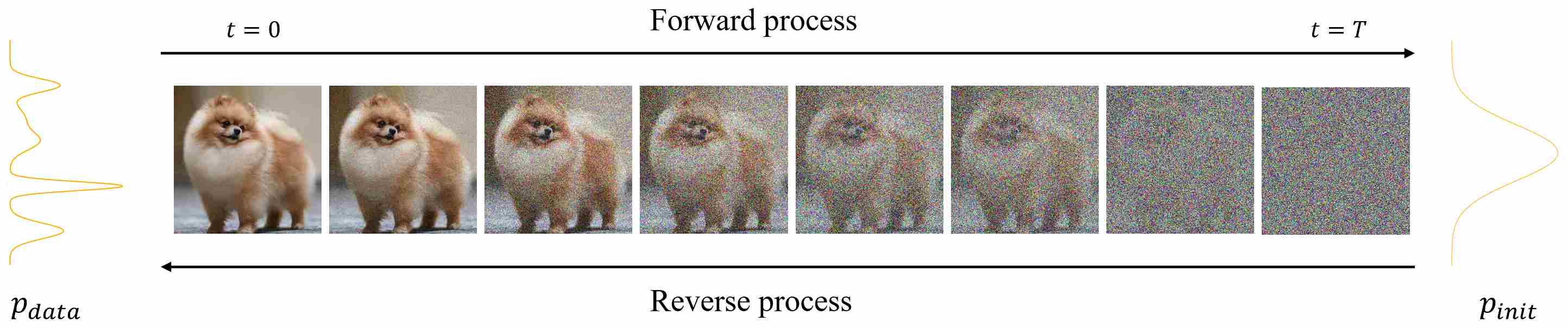
Diffusion models have been shown to be a highly promising approach in the field of image generation. They treat image generation as two independent processes: the forward process, which transforms a complex data distribution into a known prior distribution (typically a standard normal distribution) by gradually injecting noise; and the reverse process, which transforms the prior distribution back into the complex data distribution by gradually removing the noise.
The unified forward process — from a discrete perspective
In most cases, the forward process, also known as noise schedules, does not contain any learnable parameters, you only need to “manually” define it in advance. We assume that the data distribution is $p_{data}$, while the prior distribution is $p_{init}$. For any time step $t$, the noised image $x_t$ can be obtained by adding noise $\varepsilon$ ( $\varepsilon \sim p_{init}$) to a real image $x_0$ ( $x_0 \sim p_{data}$). We can formalize it as the following formula:
\[x_t=s(t)x_0+\sigma(t)\varepsilon\label{eq:1}\]Where $s(t)$ represents the signal coefficient, and $\sigma(t)$ represents the noise coefficient. The two mainstream types of noise schedules are Variance Preserving (VP) and Variance Exploding (VE).
VP: At any time step $t$, the forward (noising) process gradually decays the original signal while injecting matching noise so that the total variance stays constant (usually 1), which means that: $Var(x_t)=s(t)^2+\sigma(t)^2=1$ (assuming the data has been whitened so that $var(x_0)=1$). We can rewrite the VP-type noise scheduling with DDPM format:
\[x_t=\sqrt {\bar {\alpha_t}}x_0+ \sqrt {1-\bar {\alpha_t}} \varepsilon\label{eq:2}\]Where $s(t) = \sqrt {\bar {\alpha_t}}$ , $\sigma(t) = \sqrt {1-\bar {\alpha_t}} $. Two commonly used VP-type noise schedules include linear scheduling (DDPM1 and DDIM2) and cosine scheduling (iDDPM3)
VE: The forward process preserves the original signal intact and continuously adds noise, and eventually variance grows unbounded over time. We can rewrite the VE-type noise scheduling with NCSN 4 format:
\[x_t= x_0+ \sigma(t) \varepsilon\label{eq:3}\]The following plots compare three common forward (noising) schedules in diffusion models: VP–linear, VP–cosine (iDDPM), and VE. Each panel shows the signal coefficient $s(t)$ (how much of $x_0$ remains) and the noise coefficient $\sigma(t)$ (how much noise is injected).
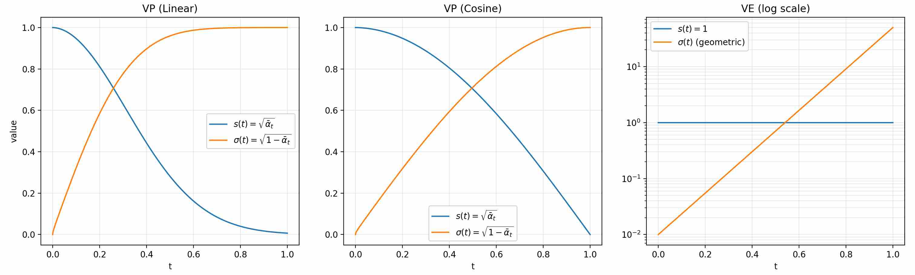
VP schedules preserve variance under a whitened-data assumption ($var(x_0)=1$), gradually trading signal for noise, compared to linear VP, cosine-VP retains more signal at late times (slower decay near $t=1$). VE keeps the signal level fixed and ramps up noise magnitude across time. Use cases often favor VP when you want a controlled signal-to-noise decay, and VE when you want broad noise scales for score matching.
From discrete perspective to continuous perspective
Diffusion models originally operate in discrete time, with a fixed number of timesteps $t=1,2,\dots,T$, as $T \to \infty$, time becomes a continuous variable $t \in [0,1]$. From this point of view, Song et al. 5 present a stochastic differential equation (SDE) to unify the existing discrete diffusion models.
Briefly speaking, the discrete noise schedule defined in formula $\ref{eq:1}$ can be formalized as
\[dx_t=f(t)x_tdt + g(t)dw_t\label{eq:4}\]The question is when given $s(t)$ and $\sigma(t)$, how can we derive the expressions for $f(t)$ and $g(t)$ , and vice versa.
By observing Equation $\ref{eq:1}$ , it is not difficult to find that $x_t$ follows a Gaussian distribution with mean $m(x_t)=s(t)x_0$ and variance $var(x_t)=\sigma(t)^2$.
\[x_t \sim \mathcal N (s(t)x_0, \sigma(t)^2 I)\label{eq:5}\]In the subsequent explanations, we will use $m(t)$ to represent the mean $m(x_t)$ and $var(t)$ to represent the variance $var(x_t)$ for convenience. Now let’s consider the SDE in continuous form ( equation \ref{eq:4}). What are its mean and variance?
First, integrate both sides of equation \ref{eq:4} from 0 to $t$ and simplify the result.
\[\begin{align} & x_t = x_0 + \int_0^tf(s)x_sds + \int_0^tg(s)dw_s\label{eq:6} \\ \Longrightarrow \ \ \ \ & \mathbb E(x_t|x_0) = \mathbb E(x_0|x_0) + \mathbb E (\int_0^tf(s)x_sds |x_0) + \mathbb E(\int_0^tg(s)dw_s|x_0)\label{eq:7} \\ \Longrightarrow \ \ \ \ & \mathbb E(x_t|x_0) = \mathbb E(x_0|x_0) + \int_0^tf(s)\mathbb E (x_s|x_0)ds + \int_0^tg(s)\mathbb E(dw_s|x_0)\label{eq:8} \end{align}\]Where $\mathbb E(x_t|x_0)$ is the mean we need to compute, let $m(t)=\mathbb E(x_t|x_0)$, according to the properties of the Wiener process, we have $\mathbb E(dw_s|x_0) =0$, take the derivative of both sides of the above equation with respect to $t$, and simplify.
\[m'(t) = f(t)m(t)\label{eq:9}\]Equation \ref{eq:9} is a simple linear ordinary differential equation, solving it directly yields $m(t)=e^{\int_0^tf(s)ds}x_0$ (the initial value is $m(0)=x_0$). Next, we need to derive the variance of SDE, according to Ito’s lemma 6,
\[\begin{align} & dx_t^2 = 2x_tdx_t + g^2(t)dt\label{eq:10} \\[10pt] \Longrightarrow \ \ \ \ & dx_t^2=2x_t(f(t)x_tdt+g(t)dw_t)+g^2(t)dt\label{eq:11} \\[10pt] \Longrightarrow \ \ \ \ & dx_t^2=(2f(t)x_t^2+g^2(t))dt+2x_tg(t)dw_t\label{eq:12} \end{align}\]integrate both sides from 0 to $t$ and simplify the result.
\[\begin{align} & x_t^2 = x_0^2 + \int_0^t(2f(s)x_s^2+g^2(s))ds + \int_0^t2x_sg(s)dw_s\label{eq:13} \\ \Longrightarrow \ \ \ \ & \mathbb E(x_t^2|x_0) = \mathbb E(x_0^2|x_0) + \mathbb E (\int_0^t(2f(t)x_t^2+g^2(t))ds |x_0) + \mathbb E(\int_0^t2x_sg(s)dw_s|x_0)\label{eq:14} \\ \Longrightarrow \ \ \ \ & \mathbb E(x_t^2|x_0) = \mathbb E(x_0^2|x_0) + \int_0^t(2f(s)\mathbb E (x_s^2|x_0)+g^2(s))ds + \int_0^t2x_sg(s)\mathbb E(dw_s|x_0)\label{eq:15} \\ \Longrightarrow \ \ \ \ & \mathbb E(x_t^2|x_0) = \mathbb E(x_0^2|x_0) + \int_0^t(2f(s)\mathbb E (x_s^2|x_0)+g^2(s))ds\label{eq:16} \end{align}\]Set $m_2(t)= \mathbb E(x_t^2|x_0) $, take the derivative of both sides of the above equation with respect to $t$, and simplify
\[m_2'(t) = 2f(t)m_2(t)+g^2(t)\label{eq:17}\]Recall the variance formula: $var(t)=m_2(t)-m(t)^2$, take derivatives on both sides, and we get $var’(t)=m_2’(t)-2m(t)m’(t) $, substitute $m_2’(t)$ into the above equation, and simplify to obtain.
\[\begin{align} & var'(t)=m_2'(t)-2m(t)m'(t)\label{eq:18} \\[10pt] \Longrightarrow \ \ \ \ & var'(t)=2f(t)m_2(t)+g^2(t)-2f(t)m^2(t)\label{eq:19} \\[10pt] \Longrightarrow \ \ \ \ & var'(t)=2f(t)(m_2(t) - m^2(t))+g^2(t)\label{eq:20} \\[10pt] \Longrightarrow \ \ \ \ & var'(t)=2f(t)var(t)+g^2(t)\label{eq:21} \end{align}\]Equation \ref{eq:21} is a first-order linear equations, by multiplying the integrating factor $e^{-2\int_0^tf(s)ds}$, let $\phi(t)=e^{\int_0^tf(s)ds}$, we can get the solution.
\[var(t)=\phi^2(t)\int_0^t \frac{g^2(s)}{\phi^2(s)}ds\label{eq:22}\]Now we have obtained the mean and variance in the form of a continuous SDE, i,e., $x_t$ satisfies:
\[x_t \sim \mathcal N (\phi(t)x_0, \phi^2(t)\int_0^t \frac{g^2(s)}{\phi^2(s)}dsI),\ \ \ \ \phi(t)=e^{\int_0^tf(s)ds}\label{eq:23}\]Compare equation \ref{eq:5} and equation \ref{eq:23}, given $s(t)$ and $\sigma(t)$, we can derive the corresponding SDE expression, which satisfies:
\[f(t)=\frac{s'(t)}{s(t)}, \ \ \ \ \ \ g^2(t)=2(\sigma(t)\sigma'(t)-\frac{s'(t)}{s(t)}\sigma^2(t))\label{eq:24}\]Similarly, given SDE expression, we can also derive the corresponding discrete forward processing, which satisfies:
\[s(t)=\phi(t)=e^{\int_0^tf(s)ds}, \ \ \ \ \ \ \sigma^2(t)=\phi^2(t)\int_0^t \frac{g^2(s)}{\phi^2(s)}ds\label{eq:25}\]Following the conclusions, we write the corresponding SDE expressions for DDPM and NCSN :
| DDPM | NCSN | |
|---|---|---|
| Discrete forward process | $x_t=\sqrt {\bar {\alpha_t}}x_0+ \sqrt {1-\bar {\alpha_t}} \varepsilon$ | $x_t= x_0+\sigma_t\varepsilon$ |
| $s(t),\ \ \sigma(t)$ | $s(t)=\sqrt {\bar {\alpha_t}}, \ \ \sigma(t)=\sqrt {1-\bar {\alpha_t}} $ | $s(t)=1, \ \ \sigma(t)=\sigma_t $ |
| $f(t),\ \ g(t)$ | $f(t)=-\frac{1}{2}\beta_t,\ \ g(t)=\sqrt {\beta_t}$ | $f(t)=0,\ \ g(t)=\sqrt {\frac{d\sigma^2_t}{dt}}$ |
| SDE | $dx_t=-\frac{1}{2}\beta_tx_tdt+\sqrt {\beta_t}dw_t$ | $dx_t=\sqrt {\frac{d\sigma^2_t}{dt}}dw_t$ |
Reverse Process
The reverse process is the opposite of the forward process, by sampling an initial point $x_T$ from the prior distribution $p_{init}$ ($x_T \sim p_{init}$), and finally generating samples $x_0 \sim p_{data}$ through continuous denoising.
According to Anderson equation7, the reverse of a diffusion process is also a diffusion process, running backwards in time and given by the reverse-time SDE:
\[dx_t=\big( f(t)x_t-g^2(t)\nabla_{x_t} \log p_t(x_t) \big)dt + g(t)d\bar w_t\label{eq:26}\]Here, $\bar w_t$, like $w_t$, is a standard Wiener process, except that the direction of $w_t$ is reversed from T to 0 (or from 1 to 0 from a continuous perspective). $\nabla_{x_t} \log p_t(x_t)$ is known as score, score refers to the gradient (with respect to $x_t$) of the log-probability density at any time step $t$.
If we know the score for any time step $t$, we can apply equation \ref{eq:26} to generate new samples by solving SDE. Song et al. 5 further point out that equation \ref{eq:26} has an equivalent ODE expression, which is also known as Probability-flow ODE (PF-ODE)
\[dx_t=\big( f(t)x_t-\frac{1}{2}g^2(t)\nabla_{x_t} \log p_t(x_t) \big)dt\label{eq:27}\]Be careful, the equivalence does not mean that the result obtained by solving equation \ref{eq:26} is the same as that obtained by solving equation \ref{eq:27}. Instead, it means that, for any time step $t$, the result obtained by solving equation \ref{eq:26} (denoted as $x_t^1$) has the same marginal probability density as the result obtained by solving equation \ref{eq:27} (denoted as $x_t^2$), i,e. $x_t^1 \sim p(x_t)$ and $x_t^2 \sim p(x_t)$.
Advantage: Thanks to the probability-flow ODE formulation, one can generate samples by integrating a deterministic ODE instead of simulating the full stochastic differential equation. Because the ODE trajectory is fully determined by its initial value, it’s easier to debug and often requires fewer function evaluations than the corresponding SDE sampler—so sampling via the ODE can be substantially faster. By contrast, SDE sampling injects fresh noise at each step, which naturally induces greater randomness (and thus diversity) in the generated outputs.
The following animation contrasts two reverse processes used in diffusion models as time runs from $t=1$ to $t=0$. The shaded quantile bands (5–95% and 25–75%) summarize thousands of reverse SDE sample paths, showing the stochastic spread over time; the dashed line is the SDE mean. The bold solid curve is the probability-flow ODE trajectory, which is deterministic and unique for the same initial condition. Despite their different dynamics (noise in SDE, none in ODE), both processes are designed to produce the same marginal distribution $p_t(x)$ at each time $t$; the animation emphasizes the difference in how they move through state space to reach those marginals.
Reading guide: the bands widen/narrow to reflect uncertainty under the SDE, the mean (dashed) may deviate from the ODE path, and the ODE curve remains smooth and single-valued throughout. (Implementation uses Euler–Maruyama for the SDE and Euler for the ODE in a simple 1D illustrative model; parameters can be adjusted to show stronger or weaker stochasticity.)
Conclusion
In this post, we have provided a unified view of the forward process in diffusion models, bridging discrete noise schedules (such as VP and VE types) with their continuous counterparts via stochastic differential equations (SDEs). We derived the relationships between signal/noise coefficients and SDE parameters, illustrated with examples from DDPM and NCSN. Additionally, we introduced the reverse process, including its SDE formulation, the score function, and the equivalent probability-flow ODE, highlighting the trade-offs between stochastic and deterministic sampling. In the next few posts, we will delve into training diffusion models through score estimation and explore efficient sampling techniques for generation.
References
Ho J, Jain A, Abbeel P. Denoising diffusion probabilistic models[J]. Advances in neural information processing systems, 2020, 33: 6840-6851. ↩
Song J, Meng C, Ermon S. Denoising diffusion implicit models[J]. arXiv preprint arXiv:2010.02502, 2020. ↩
Nichol A Q, Dhariwal P. Improved denoising diffusion probabilistic models[C]//International conference on machine learning. PMLR, 2021: 8162-8171. ↩
Song Y, Ermon S. Generative modeling by estimating gradients of the data distribution[J]. Advances in neural information processing systems, 2019, 32. ↩
Song Y, Sohl-Dickstein J, Kingma D P, et al. Score-based generative modeling through stochastic differential equations[J]. arXiv preprint arXiv:2011.13456, 2020. ↩ ↩2
Itô K. On a formula concerning stochastic differentials[J]. Nagoya Mathematical Journal, 1951, 3: 55-65. ↩
Anderson B D O. Reverse-time diffusion equation models[J]. Stochastic Processes and their Applications, 1982, 12(3): 313-326. ↩