
Unifying Discrete and Continuous Perspectives in Diffusion Models
📅 Published: | 🔄 Updated:
📘 TABLE OF CONTENTS
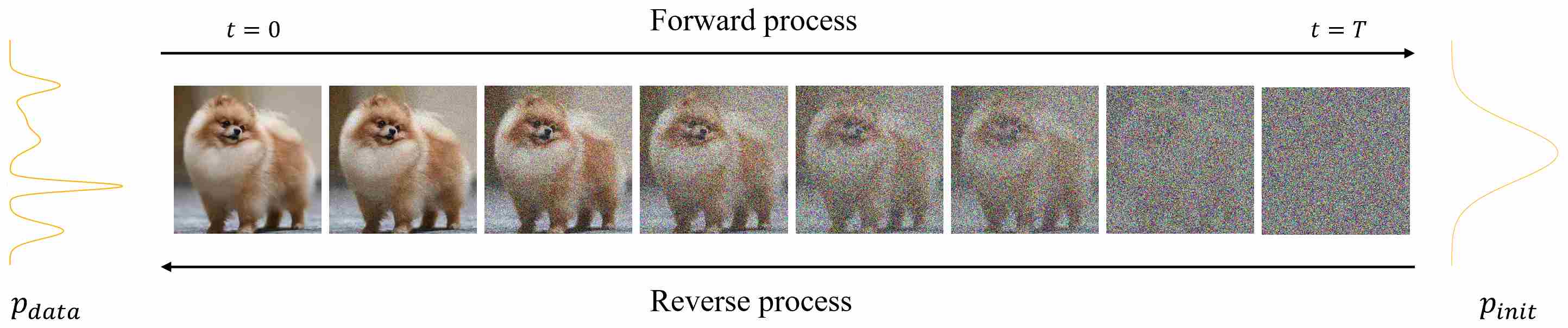
Diffusion models have emerged as one of the most powerful paradigms in modern generative AI, enabling high-fidelity image, video, and multimodal synthesis. At their core, these models are built upon a pair of complementary processes: a forward process, which gradually corrupts data by injecting noise, and a reverse process, which aims to recover the original data distribution by removing noise step by step.
1. Introduction
Traditionally, diffusion models were introduced in discrete time, where the forward process is described by a noise-scheduling formula such as
\[x_t = s(t) x_0 + \sigma(t) \epsilon,\qquad \epsilon \sim \mathcal N(0, I)\]encompassing both Variance Preserving (VP) and Variance Exploding (VE) families. This discrete viewpoint is intuitive and easy to implement, but it can sometimes obscure the deeper mathematical structure.
A more unified perspective arises when we let the number of timesteps grow large and move to continuous time. In this limit, the forward process can be equivalently expressed as a stochastic differential equation (SDE),
\[{\mathrm d}x_t = f(t)x_t {\mathrm d}t + g(t) {\mathrm d}w_t,\]where the coefficients $(s(t), \sigma(t))$ in the discrete formulation correspond directly to the continuous coefficients $(f(t), g(t))$. This bridge between discrete and continuous forms allows us to interpret and compare different diffusion models within a single coherent framework.
The story does not end with the forward process. Once we accept that the forward dynamics can be written as an SDE, a natural consequence is that the reverse dynamics must also be an SDE—augmented with a score function that captures the gradient of the log-density. This insight leads to the celebrated reverse-time SDE 1 and its deterministic counterpart, the probability-flow ODE (PF-ODE) 2. Both describe the reverse process but from slightly different perspectives: the SDE introduces stochasticity that promotes sample diversity, while the PF-ODE provides a deterministic and often more efficient path to generation.
In this article, we take a focused journey through these ideas. We deliberately avoid discussions of training objectives or sampling algorithms, and instead concentrate on the mathematical unification: how any discrete noising scheme can be systematically translated into its continuous SDE form, and how the reverse process naturally extends to both SDE and ODE formulations. By the end, we will see that diffusion models, regardless of their discrete appearance, can all be understood within this elegant continuous framework.
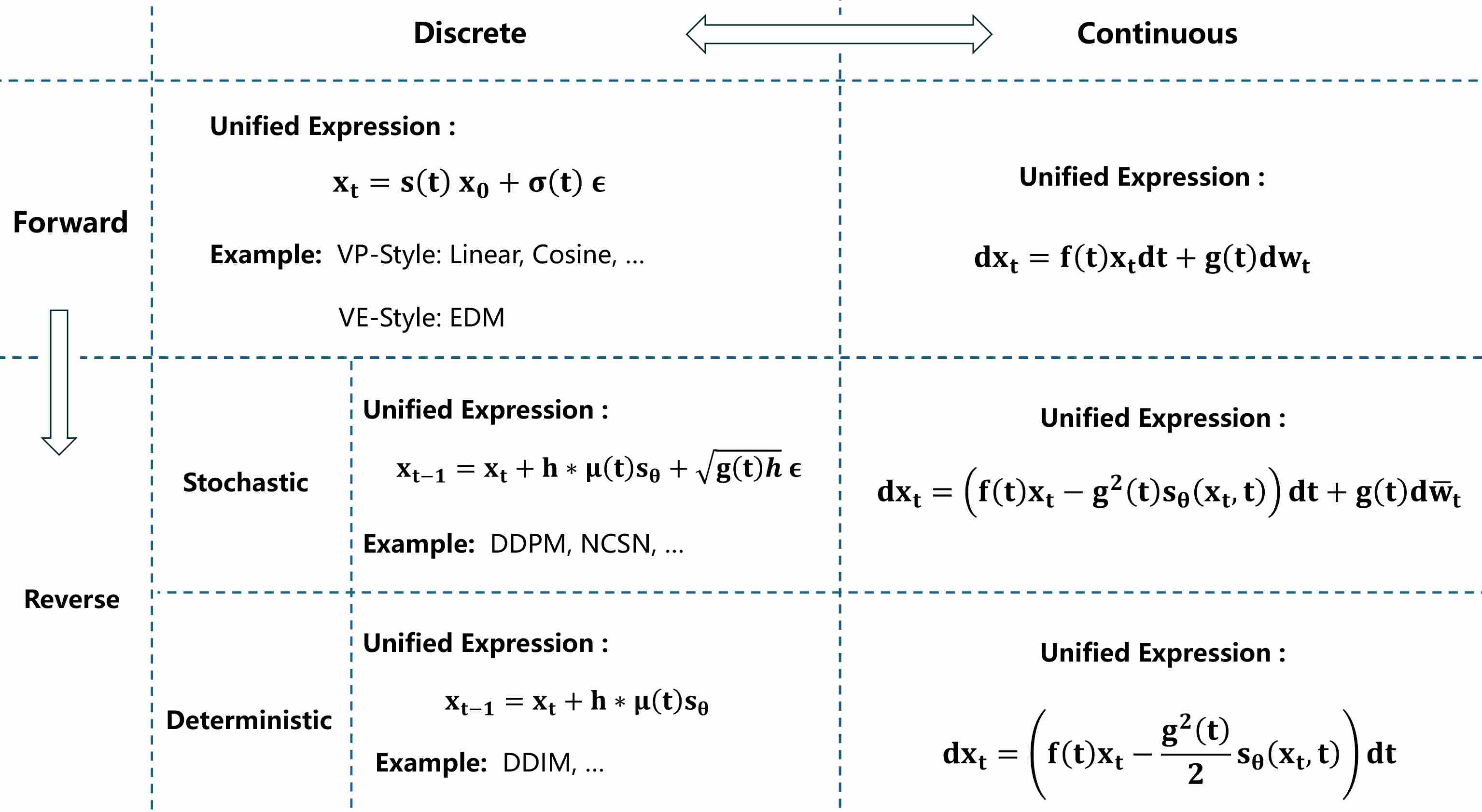
We can use a diagram to summarize the relationships between forward and reverse, discrete and continuous in diffusion models, which is also the content this article aims to explain.
2. Forward Process in Discrete Time
In most cases, the forward process, also known as noise schedules, does not contain any learnable parameters, you only need to “manually” define it in advance. We assume that the data distribution is $p_{\text{data}}$, while the prior distribution is $p_{\text{init}}$. For any time step $t$, the noised image $x_t$ can be obtained by adding noise $\epsilon$ ( $\epsilon \sim p_{\text{init}}$) to a real image $x_0$ ( $x_0 \sim p_{\text{data}}$). We can formalize it as the following formula:
\[x_t=s(t)x_0+\sigma(t)\epsilon\label{eq:1}\]Where $s(t)$ represents the signal coefficient, and $\sigma(t)$ represents the noise coefficient. The two mainstream types of noise schedules are Variance Preserving (VP) and Variance Exploding (VE).
2.1 Variance Preserving Formulation
At any time step $t$, the forward (noising) process gradually decays the original signal while injecting matching noise so that the total variance stays constant (usually 1), which means that:
\[\text{Var}(x_t)=s(t)^2+\sigma(t)^2=1\]we assume the data has been whitened so that $var(x_0)=1$. We can rewrite the VP-type noise scheduling with DDPM format:
\[x_t=\sqrt {\bar {\alpha_t}}x_0+ \sqrt {1-\bar {\alpha_t}} \epsilon\label{eq:2}\]Where $s(t) = \sqrt {\bar {\alpha_t}}$ , $\sigma(t) = \sqrt {1-\bar {\alpha_t}} $. Two commonly used VP-type noise schedules include linear scheduling (DDPM3 and DDIM4) and cosine scheduling (iDDPM5)
2.2 Variance Exploding Formulation
The forward process preserves the original signal intact and continuously adds noise, and eventually variance grows unbounded over time. We can rewrite the VE-type noise scheduling with NCSN 6 format:
\[x_t= x_0+ \sigma(t) \epsilon\label{eq:3}\]The following plots compare three common forward (noising) schedules in diffusion models: VP–linear, VP–cosine (iDDPM), and VE. Each panel shows the signal coefficient $s(t)$ (how much of $x_0$ remains) and the noise coefficient $\sigma(t)$ (how much noise is injected).
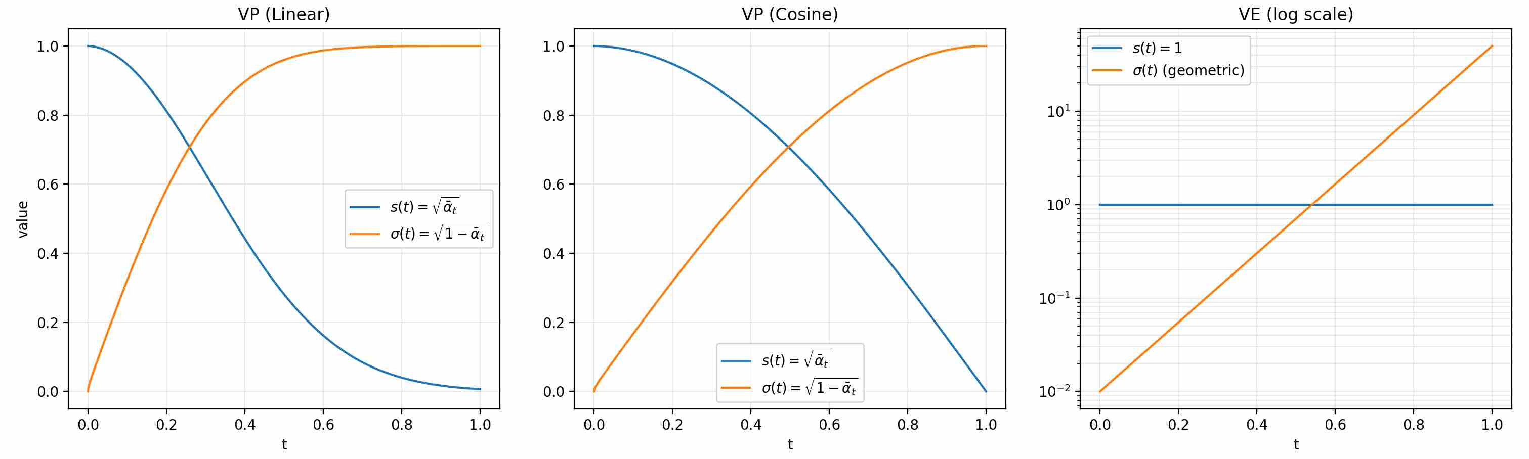
VP schedules preserve variance under a whitened-data assumption ($var(x_0)=1$), gradually trading signal for noise, compared to linear VP, cosine-VP retains more signal at late times (slower decay near $t=1$). VE keeps the signal level fixed and ramps up noise magnitude across time. Use cases often favor VP when you want a controlled signal-to-noise decay, and VE when you want broad noise scales for score matching.
3. Bridging Discrete and Continuous: Deriving the SDE Form
Diffusion models originally operate in discrete time, with a fixed number of timesteps
\[t=1,2,\dots,T\]As $T \to \infty$, time becomes a continuous variable $t \in [0,1]$. From this point of view, Song et al. 2 present a stochastic differential equation (SDE) to unify the existing discrete diffusion models.
Briefly speaking, the discrete noise schedule defined in formula $\ref{eq:1}$ can be formalized as
\[{\mathrm d}x_t=f(t)x_t{\mathrm d}t + g(t){\mathrm d}w_t\label{eq:4}\]The question is when given $s(t)$ and $\sigma(t)$, how can we derive the expressions for $f(t)$ and $g(t)$ , and vice versa.
By observing Equation $\ref{eq:1}$ , it is not difficult to find that the conditional distribution \(\{x_t \mid x_0\}\) (not $x_t$) follows a Gaussian distribution with mean $m(x_t)=s(t)x_0$ and variance $var(x_t)=\sigma(t)^2$.
\[\{x_t \mid x_0\} \sim \mathcal N \left( s(t)x_0, \sigma(t)^2\;I \right)\label{eq:5}\]In the subsequent explanations, we will use $m(t)$ to represent the mean $m(x_t)$ and $var(t)$ to represent the variance $var(x_t)$ for convenience. Now let’s consider the SDE in continuous form ( equation \ref{eq:4}). What are its mean and variance?
Takeaway: In diffusion models, the theoretical forward process defines a marginal distribution $p(x_t)$, which describes how data evolve under noise. However, this marginal is a complicated mixture of Gaussians determined by the unknown data distribution $p(x_0)$, and thus has no closed form. $$ p(x_t)=\int p(x_t \mid x_0) p_{\rm data}(x_0) {\mathbf d}x_0. $$ In practice, all derivations and training objectives rely instead on the conditional distribution $$p(x_t \mid x_0) = \mathcal N(s_t x_0, \sigma_t^2 I),$$ which is analytically tractable. By sampling $x_t$ from this conditional, we can compute losses and gradients without ever needing to explicitly represent the intractable marginal distribution.
First, integrate both sides of equation \ref{eq:4} from 0 to $t$ and simplify the result.
\[\begin{align} & x_t = x_0 + \int_0^tf(s)x_sds + \int_0^tg(s)dw_s\label{eq:6} \\[10pt] \Longrightarrow \ \ \ \ & \mathbb E(x_t|x_0) = \mathbb E(x_0|x_0) + \mathbb E \left(\int_0^tf(s)x_sds |x_0 \right) + \mathbb E \left(\int_0^tg(s)dw_s|x_0 \right)\label{eq:7} \\[10pt] \Longrightarrow \ \ \ \ & \mathbb E(x_t|x_0) = \mathbb E(x_0|x_0) + \int_0^tf(s)\mathbb E (x_s|x_0)ds + \int_0^tg(s)\mathbb E(dw_s|x_0)\label{eq:8} \end{align}\]Where $\mathbb E(x_t|x_0)$ is the mean we need to compute, let $m(t)=\mathbb E(x_t|x_0)$, according to the properties of the Wiener process, we have $\mathbb E(dw_s|x_0) =0$, take the derivative of both sides of the above equation with respect to $t$, and simplify.
\[m'(t) = f(t)\,m(t)\label{eq:9}\]Equation \ref{eq:9} is a simple linear ordinary differential equation, solving it directly yields
\[m(t)= \exp \left(\int_0^tf(s)ds \right)\;x_0,\]with the initial value is $m(0)=x_0$. Next, we need to derive the variance of SDE, according to Ito’s lemma 7, the second-order moment $d(x_t^2)$ includes both a first-order term and an Itô correction term.
\[d(x_t^2) = \underbrace{2x_t\,dx_t}_{\text{a first-order term}} + \underbrace{(g^2(t))dt}_{\text{Itô correction term}}\]Takeaway: Please notes that, unlike the standard differential rule, for a smooth deterministic function $x_t$, we have $$d(x_t^2) = 2x_t\,dx_t$$ However, when $x_t$ is a stochastic process following an Itô SDE, the differential $d(x_t^2)$ contains an correction term, the key reason is that the differential square of Brownian motion cannot be ignored $$(dw_t)^2 = dt \neq 0$$
Expand and simplify the above equation
\[\begin{align} & dx_t^2 = 2x_tdx_t + g^2(t)dt\label{eq:10} \\[10pt] \Longrightarrow \ \ \ \ & dx_t^2=2x_t(f(t)x_tdt+g(t)dw_t)+g^2(t)dt\label{eq:11} \\[10pt] \Longrightarrow \ \ \ \ & dx_t^2=(2f(t)x_t^2+g^2(t))dt+2x_tg(t)dw_t\label{eq:12} \end{align}\]integrate both sides from 0 to $t$ and simplify the result.
\[\begin{align} & x_t^2 = x_0^2 + \int_0^t \left( 2f(s)x_s^2+g^2(s) \right)ds + \int_0^t2x_sg(s)dw_s\label{eq:13} \\[10pt] \Longrightarrow \ \ \ \ & \mathbb E(x_t^2|x_0) = \mathbb E(x_0^2|x_0) + \mathbb E \left(\int_0^t(2f(t)x_t^2+g^2(t))ds |x_0 \right) + \mathbb E \left(\int_0^t2x_sg(s)dw_s|x_0 \right)\label{eq:14} \\[10pt] \Longrightarrow \ \ \ \ & \mathbb E(x_t^2|x_0) = \mathbb E(x_0^2|x_0) + \int_0^t \left( 2f(s)\mathbb E (x_s^2|x_0)+g^2(s) \right)ds + \int_0^t2x_sg(s)\mathbb E(dw_s|x_0)\label{eq:15} \\[10pt] \Longrightarrow \ \ \ \ & \mathbb E(x_t^2|x_0) = \mathbb E(x_0^2|x_0) + \int_0^t \left( 2f(s)\mathbb E (x_s^2|x_0)+g^2(s) \right)ds\label{eq:16} \end{align}\]Set $m_2(t)= \mathbb E(x_t^2|x_0) $, take the derivative of both sides of the above equation with respect to $t$, and simplify
\[m_2'(t) = 2f(t)m_2(t)+g^2(t)\label{eq:17}\]Recall the variance formula: $var(t)=m_2(t)-m(t)^2$, take derivatives on both sides, and we get $var’(t)=m_2’(t)-2m(t)m’(t) $, substitute $m_2’(t)$ into the above equation, and simplify to obtain.
\[\begin{align} & {\mathrm var}'(t)=m_2'(t)-2m(t)m'(t)\label{eq:18} \\[10pt] \Longrightarrow \ \ \ \ & {\mathrm var}'(t)=2f(t)m_2(t)+g^2(t)-2f(t)m^2(t)\label{eq:19} \\[10pt] \Longrightarrow \ \ \ \ & {\mathrm var}'(t)=2f(t)\,(m_2(t) - m^2(t))+g^2(t)\label{eq:20} \\[10pt] \Longrightarrow \ \ \ \ & {\mathrm var}'(t)=2f(t)\,{\mathrm var}(t)+g^2(t)\label{eq:21} \end{align}\]Equation \ref{eq:21} is a first-order linear equations, by multiplying the integrating factor $e^{-2\int_0^tf(s)ds}$, let $\phi(t)=e^{\int_0^tf(s)ds}$, we can get the solution.
\[var(t)=\phi^2(t)\int_0^t \frac{g^2(s)}{\phi^2(s)}ds\label{eq:22}\]Now we have obtained the mean and variance in the form of a continuous SDE, i,e., the conditional distribution \(\{x_t \mid x_0\}\) satisfies:
\[\{x_t \mid x_0\} \sim \mathcal N \left(\phi(t)x_0,\, \phi^2(t)\int_0^t \frac{g^2(s)}{\phi^2(s)}ds\;I \right), \ \ \ \phi(t)=\exp{\left(\int_0^tf(s)\;ds\right)}\label{eq:23}\]Compare equation \ref{eq:5} and equation \ref{eq:23}, given $s(t)$ and $\sigma(t)$, we can derive the corresponding SDE expression, which satisfies:
\[\begin{align} & f(t)=\frac{s'(t)}{s(t)}, \\[10pt] & g^2(t)=2\sigma^2(t) \left( \frac{\sigma'(t)}{\sigma(t)}-\frac{s'(t)}{s(t)}\right)\label{eq:24} \end{align}\]Similarly, given SDE expression, we can also derive the corresponding discrete forward processing, which satisfies:
\[\begin{align} & s(t)=\phi(t)=\exp \left({\int_0^tf(s)ds}\right), \\[10pt] & \sigma^2(t)=\phi^2(t)\int_0^t \frac{g^2(s)}{\phi^2(s)}ds\label{eq:25} \end{align}\]Following the conclusions, we write the corresponding SDE expressions for DDPM and NCSN :
| DDPM | NCSN | |
|---|---|---|
| Discrete forward process | $x_t=\sqrt {\bar {\alpha_t}}x_0+ \sqrt {1-\bar {\alpha_t}} \epsilon$ | $x_t= x_0+\sigma_t\epsilon$ |
| $s(t),\ \ \sigma(t)$ | $s(t)=\sqrt {\bar {\alpha_t}}, \ \ \sigma(t)=\sqrt {1-\bar {\alpha_t}} $ | $s(t)=1, \ \ \sigma(t)=\sigma_t $ |
| $f(t),\ \ g(t)$ | $f(t)=-\frac{1}{2}\beta(t),\ \ g(t)=\sqrt {\beta(t)}$ | $f(t)=0,\ \ g(t)=\sqrt {\frac{d\sigma^2_t}{dt}}$ |
| SDE | $dx_t=-\frac{1}{2}\beta(t)x_tdt+\sqrt {\beta(t)}dw_t$ | $dx_t=\sqrt {\frac{d\sigma^2_t}{dt}}dw_t$ |
The solution to the table above requires the transformation from discrete sequences $\beta_t$ to continuous functions $\beta(t)$, which satisfy \(\beta_t=\beta(t)\Delta t\). In the continuous-time limit, convert the discrete product into an integral.
\[\begin{align} \log \bar \alpha_t & = \log \prod_{i=1}^{t}\alpha_i = \log \prod_{i=1}^{t}(1-\beta_i)= \sum_{i=1}^t \log (1-\beta(i)\Delta i) \\[10pt] & \approx \sum_{i=1}^t \underbrace{(-\beta(i)\Delta i)}_{\text{Taylor expansion }} = - \int_0^t \beta(i)di \end{align}\]Thus, we obtain the following important equation, which is frequently used in coefficient transformations.
\[\bar \alpha_t = \exp \left(- \int_0^t \beta(i)di \right) \quad \Longrightarrow \quad (\bar \alpha_t)' = -\beta(t) \bar \alpha_t\]4. Reverse Dynamics: Reverse-Time SDE and PF-ODE
The reverse process is the opposite of the forward process, by sampling an initial point $x_T$ from the prior distribution $p_{\text{init}}$ ($x_T \sim p_{\text{init}}$), and finally generating samples $x_0 \sim p_{\text{data}}$ through continuous denoising.
According to Anderson equation1, the reverse of a diffusion process is also a diffusion process, running backwards in time and given by the reverse-time SDE:
\[dx_t=\big( f(t)x_t-g^2(t)\nabla_{x_t} \log p_t(x_t) \big)dt + g(t)d\bar w_t\label{eq:26}\]Here, $\bar w_t$, like $w_t$, is a standard Wiener process, except that the direction of $w_t$ is reversed from T to 0 (or from 1 to 0 from a continuous perspective). $\nabla_{x_t} \log p_t(x_t)$ is known as score, score refers to the gradient (with respect to $x_t$) of the log-probability density at any time step $t$.
If we know the score for any time step $t$, we can apply equation \ref{eq:26} to generate new samples by solving SDE. Song et al. 2 further point out that equation \ref{eq:26} has an equivalent ODE expression, which is also known as Probability-flow ODE (PF-ODE)
\[dx_t=\left( f(t)x_t-\frac{1}{2}g^2(t)\nabla_{x_t} \log p_t(x_t) \right)dt\label{eq:27}\]Be careful, the equivalence does not mean that the result obtained by solving equation \ref{eq:26} is the same as that obtained by solving equation \ref{eq:27}. Instead, it means that, for any time step $t$, the result obtained by solving equation \ref{eq:26} (denoted as $x_t^1$) has the same marginal probability density as the result obtained by solving equation \ref{eq:27} (denoted as $x_t^2$), i,e.
\[x_t^1 \sim p(x_t)\,\, \text{and}\,\, x_t^2 \sim p(x_t),\qquad x_t^1 \neq x_t^2.\]Advantage: Thanks to the probability-flow ODE formulation, one can generate samples by integrating a deterministic ODE instead of simulating the full stochastic differential equation. Because the ODE trajectory is fully determined by its initial value, it’s easier to debug and often requires fewer function evaluations than the corresponding SDE sampler—so sampling via the ODE can be substantially faster. By contrast, SDE sampling injects fresh noise at each step, which naturally induces greater randomness (and thus diversity) in the generated outputs.
The following animation contrasts two reverse processes used in diffusion models as time runs from $t=1$ to $t=0$. The shaded quantile bands (5–95% and 25–75%) summarize thousands of reverse SDE sample paths, showing the stochastic spread over time; the dashed line is the SDE mean. The bold solid curve is the probability-flow ODE trajectory, which is deterministic and unique for the same initial condition. Despite their different dynamics (noise in SDE, none in ODE), both processes are designed to produce the same marginal distribution $p_t(x)$ at each time $t$; the animation emphasizes the difference in how they move through state space to reach those marginals.
Reading guide: the bands widen/narrow to reflect uncertainty under the SDE, the mean (dashed) may deviate from the ODE path, and the ODE curve remains smooth and single-valued throughout. (Implementation uses Euler–Maruyama (EM) for the SDE and Euler for the ODE in a simple 1D illustrative model; parameters can be adjusted to show stronger or weaker stochasticity.)
4.1 Verify DDPM Reverse Process as Reverse SDE Family
Given $f(t)=-1/2\beta(t)$ and $g(t)=\sqrt{\beta(t)}$, we can derive DDPM reverse SDE.
\[\begin{align} dx_t & =\left( f(t)x_t - g(t)^2s_{\theta}(x_t, t)\right) dt + g(t)dw_t \\[10pt] & = \left( -\frac{1}{2}\beta(t)x_t - \beta(t)s_{\theta}(x_t, t)\right) dt + \sqrt{\beta(t)}dw_t \end{align}\]Let $t$ be the current time and $t-1$ the next (earlier) time, set $\Delta t$ is step size. a backward Euler–Maruyama (EM) step for the reverse SDE reads
\[x_{t-1} \;\approx\; x_t \;+\; \Big(\frac{1}{2}\beta(t)x_t + \beta(t)s_{\theta}(x_t, t)\Big){\Delta t}\, \;+\;\sqrt{\beta(t)\,{\Delta t}}\;z,\quad z\sim\mathcal N(0,I),\]where we used that moving backward in $t$ flips the sign of $dt$ (hence the “$+$” above). When step size $\Delta t$ is small, we have $\beta_t \approx \beta(t)\,\Delta t$,
\[\begin{align} x_{t-1} \;& \approx\; x_t \;+\; \Big(\frac{1}{2}\beta_tx_t + \beta_ts_{\theta}(x_t, t)\Big)\, \;+\;\sqrt{\beta_t}\;z \\[10pt] & \approx\; x_t \;+\; \frac{1}{2}\beta_tx_t + \beta_ts_{\theta}(x_t, t)\,+\frac{1}{2}{\beta_t^2}s_{\theta}(x_t, t)\;+\;\sqrt{\beta_t}\;z \\[10pt] & \approx\; \left( 1 \;+\; \frac{1}{2}\beta_t \right)x_t + \left( 1 \;+\; \frac{1}{2}\beta_t \right)\beta_ts_{\theta}(x_t, t)\,\;+\;\sqrt{\beta_t}\;z \\[10pt] & = \; \left( 1 \;+\; \frac{1}{2}\beta_t \right)(x_t + {\beta_t}s_{\theta}(x_t, t))\,\;+\;\sqrt{\beta_t}\;z \end{align}\]Substituting $s_\theta= -\epsilon_\theta/\sqrt{1-\bar\alpha_t}$ gives
\[x_{t-1} = \; \left( 1 \;+\; \frac{1}{2}\beta_t \right)(x_t - \frac{\beta_t}{\sqrt{1-\bar\alpha_t}}\epsilon_{\theta}(x_t, t))\,\;+\;\sqrt{\beta_t}\;z\]Now compare this with DDPM’s discrete reverse formulation:
\[x_{t-1} \;=\; \frac{1}{\sqrt{\alpha_t}} \Big( x_t - \frac{\beta_t}{\sqrt{1-\bar\alpha_t}}\;\epsilon_\theta(x_t,t)\Big) + \sqrt{\beta_t \frac{1-\bar \alpha_{t-1}}{1- \bar \alpha_t}}\;z.\]Let us perform the Taylor expansion for $ \sqrt{\alpha_t} $
\[\begin{align} \frac{1}{\sqrt{\alpha_t}} & = (1-\beta_t)^{-1/2} = (1-\beta(t)\Delta t)^{-1/2} \\[10pt] & =\; 1+\frac{1}{2}\beta(t)\Delta t + O({\Delta t}^2) \approx 1+\frac{1}{2}\beta_t \end{align}\]The coefficients of both functions satisfy the first-order Taylor approximation, their difference is of order $ O({\Delta t}^2) $, so when $ \Delta t $ is very small, they can be considered equal. Thus the DDPM mean is exactly the Euler–Maruyama drift step of the reverse VP-SDE (first-order accurate).
When it comes to Noise variance.
\[\beta_t\frac{1-\bar\alpha_{t-1}}{1-\bar\alpha_t} = \beta_t\frac{1-\bar\alpha_{t-1}}{1-{\bar\alpha_{t-1}}{\alpha_t}} = \beta_t\frac{1-\bar\alpha_{t-1}}{1-{\bar\alpha_{t-1}}{(1-\beta(t)\Delta t)}}\]when step size $ \Delta t $ is very small, the DDPM variance matches the Euler–Maruyama diffusion variance $\beta_t$ .
4.2 Verify NCSN Reverse Process as Reverse SDE Family
Given $f(t)=0$ and $g(t)=\sqrt{d\sigma_t^2/dt}$, we can derive NCSN reverse SDE.
\[\begin{align} dx_t & =\left( f(t)x_t - g(t)^2s_{\theta}(x_t, t)\right) dt + g(t)dw_t \\[10pt] & = \left( - \frac{d\sigma_t^2}{dt}s_{\theta}(x_t, t)\right) dt + \sqrt{\frac{d\sigma_t^2}{dt}}dw_t \end{align}\]Let $t$ be the current time and $t-1$ the next (earlier) time, set $\Delta t$ is step size. a backward Euler–Maruyama step for the reverse SDE gives
\[x_{t-1} \;\approx\; x_t \;+\; \frac{d\sigma_t^2}{dt}s_{\theta}(x_t, t){\Delta t}\, \;+ \sqrt{\frac{d\sigma_t^2}{dt}\,\Delta t}\,z,\quad z\sim\mathcal N(0,I),\]where the “$+$” again comes from stepping backward in $t$. Define the per-level step size $\alpha_t$.
\[\alpha_t \;\triangleq\; \frac{d\sigma_t^2}{dt}\,\Delta t\]then the update becomes
\[x_{t-1} \;\approx\; x_t \;+\; \alpha_t\,s_\theta(x_t,t) \;+\; \sqrt{\alpha_t}\;z.\]This is exactly the annealed Langevin step used in NCSN 6. In other words, NCSN’s sampler is the first-order EM discretization of the reverse VE-SDE at the chosen noise level $\sigma_t$.
4.3 Verify DDIM Reverse Process as PF-ODE
Recall DDIM 4 one-step sampling formulation, from $t$ to an earlier $s < t$.
\[x_s = \sqrt{\bar\alpha_s}\hat x_0 + \sqrt{1-\bar\alpha_s-\eta}\,\epsilon(x_t, t) + \eta z,\quad z \sim \mathcal{N}(0,I)\]where
\[\hat x_0 = \frac{x_t - \sqrt{1-\bar\alpha_t}\epsilon(x_t, t)}{\sqrt{\bar\alpha_t}}\]the parameter $\eta$ controls how much stochasticity is injected during sampling. Specifically, when $\eta=0$, the update becomes fully deterministic. In this section, we prove this corresponds exactly a discretization of the PF-ODE.
Let $s=t-h$ with $h\downarrow 0$. Write $\bar\alpha_t=\bar\alpha(t)$. Rewrite the DDIM step as
\[x_s =\sqrt{\frac{\bar\alpha(s)}{\bar\alpha(t)}}\,x_t +\Big(\sqrt{1-\bar\alpha(s)}-\sqrt{\frac{\bar\alpha(s)}{\bar\alpha(t)}}\,\sqrt{1-\bar\alpha_t}\Big)\epsilon_\theta(x_t,t)\label{eq:49}\]Using
\[\sqrt{\frac{\bar\alpha(s)}{\bar\alpha(t)}} = \exp\!\Big(\frac{1}{2}\!\int_{t}^{t-h}\!\!\beta(u)\,du\Big) =\; \underbrace{1+\frac{1}{2}\beta(t)h+O(h^2)}_{\text{first-order Taylor expansion}}\label{eq:50}\]and
\[\begin{align} \sqrt{1-\bar\alpha(s)} & =\sqrt{1-\bar\alpha(t-h)} = \sqrt{1-\bar\alpha(t)} - \left( \sqrt{1-\bar\alpha(t)} \right) ^{'}\,h + O(h^2) \\[10pt] & = \sqrt{1-\bar\alpha(t)} - \frac{\beta(t)\bar\alpha(t)}{2\sqrt{1-\bar\alpha(t)}}h + O(h^2)\label{eq:52} \end{align}\]Substituting \ref{eq:50} and \ref{eq:52} into \ref{eq:49}.
\[\begin{align} x_s & =\sqrt{\frac{\bar\alpha(s)}{\bar\alpha(t)}}\,x_t +\Big(\sqrt{1-\bar\alpha(s)}-\sqrt{\frac{\bar\alpha(s)}{\bar\alpha(t)}}\,\sqrt{1-\bar\alpha_t}\Big)\epsilon_\theta(x_t,t) \\[10pt] & \approx x_t + \frac{1}{2}\beta(t)h\,x_t \;-\; \frac{\beta(t)h}{2\sqrt{1-\bar\alpha_t}}\;\epsilon_\theta(x_t,t) \end{align}\]Move $x_t$ to the left while extracting $h$ from the right, yields
\[x_s - x_t = \left(\frac{1}{2}\beta(t)\,x_t \;-\; \frac{\beta(t)}{2\sqrt{1-\bar\alpha_t}}\;\epsilon_\theta(x_t,t)\right)\,h\]Compare with PF-ODE (Eq. \ref{eq:27}), one backward Euler step for the PF-ODE gives
\[\begin{align} x_s & = x_t + \big( \frac{1}{2}\beta(t)x_t+\frac{1}{2}\beta(t)\nabla_{x_t} \log p_t(x_t) \big)\,h \\[10pt] & = x_t + \big( \frac{1}{2}\beta(t)x_t-\frac{\beta(t)}{2\sqrt{1-\bar\alpha_t}}\epsilon_{\theta}(x_t, t)\big)\,h \end{align}\]DDIM’s one-step update matches PF-ODE vector field, hence, DDIM ($\eta=0$) is a consistent first-order discretization of the PF-ODE.
5. Conclusion: The Value of a Unified Perspective
In this post, we have explored diffusion models from a unified mathematical perspective, showing how the forward and reverse processes can be consistently described across both discrete and continuous formulations. The significance of this unification goes beyond mathematical elegance:
Clarity: It reveals that DDPM, DDIM, NCSN, and other variants are not isolated constructions, but instances of the same SDE family.
Flexibility: One can design or analyze noise schedules in either discrete or continuous form, depending on convenience.
Foundations for practice: The reverse SDE and PF-ODE highlight the duality between stochastic and deterministic sampling, providing the theoretical basis for modern solvers and efficiency improvements.
Convenient: In real implementations, the forward noising process is always defined discretely. Thanks to the unified framework, we can immediately translate such discrete definitions into their corresponding reverse-time SDE or PF-ODE formulations. This means that, once a score model is trained, the entire sampling process reduces to solving an SDE or ODE, making the connection to numerical solvers both direct and convenient.
In short, any discrete noising scheme can be systematically translated into its forward SDE, reverse SDE, and PF-ODE counterparts. This unified view not only sharpens theoretical understanding but also lays the groundwork for future exploration — whether in designing new schedules, improving training stability, or developing faster and more robust samplers.
6. References
Anderson B D O. Reverse-time diffusion equation models[J]. Stochastic Processes and their Applications, 1982, 12(3): 313-326. ↩ ↩2
Song Y, Sohl-Dickstein J, Kingma D P, et al. Score-based generative modeling through stochastic differential equations[J]. arXiv preprint arXiv:2011.13456, 2020. ↩ ↩2 ↩3
Ho J, Jain A, Abbeel P. Denoising diffusion probabilistic models[J]. Advances in neural information processing systems, 2020, 33: 6840-6851. ↩
Song J, Meng C, Ermon S. Denoising diffusion implicit models[J]. arXiv preprint arXiv:2010.02502, 2020. ↩ ↩2
Nichol A Q, Dhariwal P. Improved denoising diffusion probabilistic models[C]//International conference on machine learning. PMLR, 2021: 8162-8171. ↩
Song Y, Ermon S. Generative modeling by estimating gradients of the data distribution[J]. Advances in neural information processing systems, 2019, 32. ↩ ↩2
Itô K. On a formula concerning stochastic differentials[J]. Nagoya Mathematical Journal, 1951, 3: 55-65. ↩